Inverse kinematics

Kinematic task¶

Let us consider the task of bringing a point $\def\bfA{\boldsymbol{A}} \def\bfB{\boldsymbol{B}} \def\bfC{\boldsymbol{C}} \def\bfD{\boldsymbol{D}} \def\bfE{\boldsymbol{E}} \def\bfF{\boldsymbol{F}} \def\bfG{\boldsymbol{G}} \def\bfH{\boldsymbol{H}} \def\bfI{\boldsymbol{I}} \def\bfJ{\boldsymbol{J}} \def\bfK{\boldsymbol{K}} \def\bfL{\boldsymbol{L}} \def\bfM{\boldsymbol{M}} \def\bfN{\boldsymbol{N}} \def\bfO{\boldsymbol{O}} \def\bfP{\boldsymbol{P}} \def\bfQ{\boldsymbol{Q}} \def\bfR{\boldsymbol{R}} \def\bfS{\boldsymbol{S}} \def\bfT{\boldsymbol{T}} \def\bfU{\boldsymbol{U}} \def\bfV{\boldsymbol{V}} \def\bfW{\boldsymbol{W}} \def\bfX{\boldsymbol{X}} \def\bfY{\boldsymbol{Y}} \def\bfZ{\boldsymbol{Z}} \def\bfalpha{\boldsymbol{\alpha}} \def\bfa{\boldsymbol{a}} \def\bfbeta{\boldsymbol{\beta}} \def\bfb{\boldsymbol{b}} \def\bfcd{\dot{\bfc}} \def\bfchi{\boldsymbol{\chi}} \def\bfc{\boldsymbol{c}} \def\bfd{\boldsymbol{d}} \def\bfe{\boldsymbol{e}} \def\bff{\boldsymbol{f}} \def\bfgamma{\boldsymbol{\gamma}} \def\bfg{\boldsymbol{g}} \def\bfh{\boldsymbol{h}} \def\bfi{\boldsymbol{i}} \def\bfj{\boldsymbol{j}} \def\bfk{\boldsymbol{k}} \def\bflambda{\boldsymbol{\lambda}} \def\bfl{\boldsymbol{l}} \def\bfm{\boldsymbol{m}} \def\bfn{\boldsymbol{n}} \def\bfomega{\boldsymbol{\omega}} \def\bfone{\boldsymbol{1}} \def\bfo{\boldsymbol{o}} \def\bfpdd{\ddot{\bfp}} \def\bfpd{\dot{\bfp}} \def\bfphi{\boldsymbol{\phi}} \def\bfp{\boldsymbol{p}} \def\bfq{\boldsymbol{q}} \def\bfr{\boldsymbol{r}} \def\bfsigma{\boldsymbol{\sigma}} \def\bfs{\boldsymbol{s}} \def\bftau{\boldsymbol{\tau}} \def\bftheta{\boldsymbol{\theta}} \def\bft{\boldsymbol{t}} \def\bfu{\boldsymbol{u}} \def\bfv{\boldsymbol{v}} \def\bfw{\boldsymbol{w}} \def\bfxi{\boldsymbol{\xi}} \def\bfx{\boldsymbol{x}} \def\bfy{\boldsymbol{y}} \def\bfzero{\boldsymbol{0}} \def\bfz{\boldsymbol{z}} \def\defeq{\stackrel{\mathrm{def}}{=}} \def\p{\boldsymbol{p}} \def\qdd{\ddot{\bfq}} \def\qd{\dot{\bfq}} \def\q{\boldsymbol{q}} \def\xd{\dot{x}} \def\yd{\dot{y}} \def\zd{\dot{z}} \bfp$, located on one of the robot’s links, to a goal position $\def\bfA{\boldsymbol{A}} \def\bfB{\boldsymbol{B}} \def\bfC{\boldsymbol{C}} \def\bfD{\boldsymbol{D}} \def\bfE{\boldsymbol{E}} \def\bfF{\boldsymbol{F}} \def\bfG{\boldsymbol{G}} \def\bfH{\boldsymbol{H}} \def\bfI{\boldsymbol{I}} \def\bfJ{\boldsymbol{J}} \def\bfK{\boldsymbol{K}} \def\bfL{\boldsymbol{L}} \def\bfM{\boldsymbol{M}} \def\bfN{\boldsymbol{N}} \def\bfO{\boldsymbol{O}} \def\bfP{\boldsymbol{P}} \def\bfQ{\boldsymbol{Q}} \def\bfR{\boldsymbol{R}} \def\bfS{\boldsymbol{S}} \def\bfT{\boldsymbol{T}} \def\bfU{\boldsymbol{U}} \def\bfV{\boldsymbol{V}} \def\bfW{\boldsymbol{W}} \def\bfX{\boldsymbol{X}} \def\bfY{\boldsymbol{Y}} \def\bfZ{\boldsymbol{Z}} \def\bfalpha{\boldsymbol{\alpha}} \def\bfa{\boldsymbol{a}} \def\bfbeta{\boldsymbol{\beta}} \def\bfb{\boldsymbol{b}} \def\bfcd{\dot{\bfc}} \def\bfchi{\boldsymbol{\chi}} \def\bfc{\boldsymbol{c}} \def\bfd{\boldsymbol{d}} \def\bfe{\boldsymbol{e}} \def\bff{\boldsymbol{f}} \def\bfgamma{\boldsymbol{\gamma}} \def\bfg{\boldsymbol{g}} \def\bfh{\boldsymbol{h}} \def\bfi{\boldsymbol{i}} \def\bfj{\boldsymbol{j}} \def\bfk{\boldsymbol{k}} \def\bflambda{\boldsymbol{\lambda}} \def\bfl{\boldsymbol{l}} \def\bfm{\boldsymbol{m}} \def\bfn{\boldsymbol{n}} \def\bfomega{\boldsymbol{\omega}} \def\bfone{\boldsymbol{1}} \def\bfo{\boldsymbol{o}} \def\bfpdd{\ddot{\bfp}} \def\bfpd{\dot{\bfp}} \def\bfphi{\boldsymbol{\phi}} \def\bfp{\boldsymbol{p}} \def\bfq{\boldsymbol{q}} \def\bfr{\boldsymbol{r}} \def\bfsigma{\boldsymbol{\sigma}} \def\bfs{\boldsymbol{s}} \def\bftau{\boldsymbol{\tau}} \def\bftheta{\boldsymbol{\theta}} \def\bft{\boldsymbol{t}} \def\bfu{\boldsymbol{u}} \def\bfv{\boldsymbol{v}} \def\bfw{\boldsymbol{w}} \def\bfxi{\boldsymbol{\xi}} \def\bfx{\boldsymbol{x}} \def\bfy{\boldsymbol{y}} \def\bfzero{\boldsymbol{0}} \def\bfz{\boldsymbol{z}} \def\defeq{\stackrel{\mathrm{def}}{=}} \def\p{\boldsymbol{p}} \def\qdd{\ddot{\bfq}} \def\qd{\dot{\bfq}} \def\q{\boldsymbol{q}} \def\xd{\dot{x}} \def\yd{\dot{y}} \def\zd{\dot{z}} \bfp^*$, both point coordinates being expressed in the world frame. When the robot is in configuration $\def\bfA{\boldsymbol{A}} \def\bfB{\boldsymbol{B}} \def\bfC{\boldsymbol{C}} \def\bfD{\boldsymbol{D}} \def\bfE{\boldsymbol{E}} \def\bfF{\boldsymbol{F}} \def\bfG{\boldsymbol{G}} \def\bfH{\boldsymbol{H}} \def\bfI{\boldsymbol{I}} \def\bfJ{\boldsymbol{J}} \def\bfK{\boldsymbol{K}} \def\bfL{\boldsymbol{L}} \def\bfM{\boldsymbol{M}} \def\bfN{\boldsymbol{N}} \def\bfO{\boldsymbol{O}} \def\bfP{\boldsymbol{P}} \def\bfQ{\boldsymbol{Q}} \def\bfR{\boldsymbol{R}} \def\bfS{\boldsymbol{S}} \def\bfT{\boldsymbol{T}} \def\bfU{\boldsymbol{U}} \def\bfV{\boldsymbol{V}} \def\bfW{\boldsymbol{W}} \def\bfX{\boldsymbol{X}} \def\bfY{\boldsymbol{Y}} \def\bfZ{\boldsymbol{Z}} \def\bfalpha{\boldsymbol{\alpha}} \def\bfa{\boldsymbol{a}} \def\bfbeta{\boldsymbol{\beta}} \def\bfb{\boldsymbol{b}} \def\bfcd{\dot{\bfc}} \def\bfchi{\boldsymbol{\chi}} \def\bfc{\boldsymbol{c}} \def\bfd{\boldsymbol{d}} \def\bfe{\boldsymbol{e}} \def\bff{\boldsymbol{f}} \def\bfgamma{\boldsymbol{\gamma}} \def\bfg{\boldsymbol{g}} \def\bfh{\boldsymbol{h}} \def\bfi{\boldsymbol{i}} \def\bfj{\boldsymbol{j}} \def\bfk{\boldsymbol{k}} \def\bflambda{\boldsymbol{\lambda}} \def\bfl{\boldsymbol{l}} \def\bfm{\boldsymbol{m}} \def\bfn{\boldsymbol{n}} \def\bfomega{\boldsymbol{\omega}} \def\bfone{\boldsymbol{1}} \def\bfo{\boldsymbol{o}} \def\bfpdd{\ddot{\bfp}} \def\bfpd{\dot{\bfp}} \def\bfphi{\boldsymbol{\phi}} \def\bfp{\boldsymbol{p}} \def\bfq{\boldsymbol{q}} \def\bfr{\boldsymbol{r}} \def\bfsigma{\boldsymbol{\sigma}} \def\bfs{\boldsymbol{s}} \def\bftau{\boldsymbol{\tau}} \def\bftheta{\boldsymbol{\theta}} \def\bft{\boldsymbol{t}} \def\bfu{\boldsymbol{u}} \def\bfv{\boldsymbol{v}} \def\bfw{\boldsymbol{w}} \def\bfxi{\boldsymbol{\xi}} \def\bfx{\boldsymbol{x}} \def\bfy{\boldsymbol{y}} \def\bfzero{\boldsymbol{0}} \def\bfz{\boldsymbol{z}} \def\defeq{\stackrel{\mathrm{def}}{=}} \def\p{\boldsymbol{p}} \def\qdd{\ddot{\bfq}} \def\qd{\dot{\bfq}} \def\q{\boldsymbol{q}} \def\xd{\dot{x}} \def\yd{\dot{y}} \def\zd{\dot{z}} \bfq$, the (position) residual of this task is:

The goal of the task is to bring this residual to zero. Next, from forward kinematics we know how to compute the Jacobian matrix of $\def\bfA{\boldsymbol{A}} \def\bfB{\boldsymbol{B}} \def\bfC{\boldsymbol{C}} \def\bfD{\boldsymbol{D}} \def\bfE{\boldsymbol{E}} \def\bfF{\boldsymbol{F}} \def\bfG{\boldsymbol{G}} \def\bfH{\boldsymbol{H}} \def\bfI{\boldsymbol{I}} \def\bfJ{\boldsymbol{J}} \def\bfK{\boldsymbol{K}} \def\bfL{\boldsymbol{L}} \def\bfM{\boldsymbol{M}} \def\bfN{\boldsymbol{N}} \def\bfO{\boldsymbol{O}} \def\bfP{\boldsymbol{P}} \def\bfQ{\boldsymbol{Q}} \def\bfR{\boldsymbol{R}} \def\bfS{\boldsymbol{S}} \def\bfT{\boldsymbol{T}} \def\bfU{\boldsymbol{U}} \def\bfV{\boldsymbol{V}} \def\bfW{\boldsymbol{W}} \def\bfX{\boldsymbol{X}} \def\bfY{\boldsymbol{Y}} \def\bfZ{\boldsymbol{Z}} \def\bfalpha{\boldsymbol{\alpha}} \def\bfa{\boldsymbol{a}} \def\bfbeta{\boldsymbol{\beta}} \def\bfb{\boldsymbol{b}} \def\bfcd{\dot{\bfc}} \def\bfchi{\boldsymbol{\chi}} \def\bfc{\boldsymbol{c}} \def\bfd{\boldsymbol{d}} \def\bfe{\boldsymbol{e}} \def\bff{\boldsymbol{f}} \def\bfgamma{\boldsymbol{\gamma}} \def\bfg{\boldsymbol{g}} \def\bfh{\boldsymbol{h}} \def\bfi{\boldsymbol{i}} \def\bfj{\boldsymbol{j}} \def\bfk{\boldsymbol{k}} \def\bflambda{\boldsymbol{\lambda}} \def\bfl{\boldsymbol{l}} \def\bfm{\boldsymbol{m}} \def\bfn{\boldsymbol{n}} \def\bfomega{\boldsymbol{\omega}} \def\bfone{\boldsymbol{1}} \def\bfo{\boldsymbol{o}} \def\bfpdd{\ddot{\bfp}} \def\bfpd{\dot{\bfp}} \def\bfphi{\boldsymbol{\phi}} \def\bfp{\boldsymbol{p}} \def\bfq{\boldsymbol{q}} \def\bfr{\boldsymbol{r}} \def\bfsigma{\boldsymbol{\sigma}} \def\bfs{\boldsymbol{s}} \def\bftau{\boldsymbol{\tau}} \def\bftheta{\boldsymbol{\theta}} \def\bft{\boldsymbol{t}} \def\bfu{\boldsymbol{u}} \def\bfv{\boldsymbol{v}} \def\bfw{\boldsymbol{w}} \def\bfxi{\boldsymbol{\xi}} \def\bfx{\boldsymbol{x}} \def\bfy{\boldsymbol{y}} \def\bfzero{\boldsymbol{0}} \def\bfz{\boldsymbol{z}} \def\defeq{\stackrel{\mathrm{def}}{=}} \def\p{\boldsymbol{p}} \def\qdd{\ddot{\bfq}} \def\qd{\dot{\bfq}} \def\q{\boldsymbol{q}} \def\xd{\dot{x}} \def\yd{\dot{y}} \def\zd{\dot{z}} \bfp$:

which maps joint velocities $\def\bfA{\boldsymbol{A}} \def\bfB{\boldsymbol{B}} \def\bfC{\boldsymbol{C}} \def\bfD{\boldsymbol{D}} \def\bfE{\boldsymbol{E}} \def\bfF{\boldsymbol{F}} \def\bfG{\boldsymbol{G}} \def\bfH{\boldsymbol{H}} \def\bfI{\boldsymbol{I}} \def\bfJ{\boldsymbol{J}} \def\bfK{\boldsymbol{K}} \def\bfL{\boldsymbol{L}} \def\bfM{\boldsymbol{M}} \def\bfN{\boldsymbol{N}} \def\bfO{\boldsymbol{O}} \def\bfP{\boldsymbol{P}} \def\bfQ{\boldsymbol{Q}} \def\bfR{\boldsymbol{R}} \def\bfS{\boldsymbol{S}} \def\bfT{\boldsymbol{T}} \def\bfU{\boldsymbol{U}} \def\bfV{\boldsymbol{V}} \def\bfW{\boldsymbol{W}} \def\bfX{\boldsymbol{X}} \def\bfY{\boldsymbol{Y}} \def\bfZ{\boldsymbol{Z}} \def\bfalpha{\boldsymbol{\alpha}} \def\bfa{\boldsymbol{a}} \def\bfbeta{\boldsymbol{\beta}} \def\bfb{\boldsymbol{b}} \def\bfcd{\dot{\bfc}} \def\bfchi{\boldsymbol{\chi}} \def\bfc{\boldsymbol{c}} \def\bfd{\boldsymbol{d}} \def\bfe{\boldsymbol{e}} \def\bff{\boldsymbol{f}} \def\bfgamma{\boldsymbol{\gamma}} \def\bfg{\boldsymbol{g}} \def\bfh{\boldsymbol{h}} \def\bfi{\boldsymbol{i}} \def\bfj{\boldsymbol{j}} \def\bfk{\boldsymbol{k}} \def\bflambda{\boldsymbol{\lambda}} \def\bfl{\boldsymbol{l}} \def\bfm{\boldsymbol{m}} \def\bfn{\boldsymbol{n}} \def\bfomega{\boldsymbol{\omega}} \def\bfone{\boldsymbol{1}} \def\bfo{\boldsymbol{o}} \def\bfpdd{\ddot{\bfp}} \def\bfpd{\dot{\bfp}} \def\bfphi{\boldsymbol{\phi}} \def\bfp{\boldsymbol{p}} \def\bfq{\boldsymbol{q}} \def\bfr{\boldsymbol{r}} \def\bfsigma{\boldsymbol{\sigma}} \def\bfs{\boldsymbol{s}} \def\bftau{\boldsymbol{\tau}} \def\bftheta{\boldsymbol{\theta}} \def\bft{\boldsymbol{t}} \def\bfu{\boldsymbol{u}} \def\bfv{\boldsymbol{v}} \def\bfw{\boldsymbol{w}} \def\bfxi{\boldsymbol{\xi}} \def\bfx{\boldsymbol{x}} \def\bfy{\boldsymbol{y}} \def\bfzero{\boldsymbol{0}} \def\bfz{\boldsymbol{z}} \def\defeq{\stackrel{\mathrm{def}}{=}} \def\p{\boldsymbol{p}} \def\qdd{\ddot{\bfq}} \def\qd{\dot{\bfq}} \def\q{\boldsymbol{q}} \def\xd{\dot{x}} \def\yd{\dot{y}} \def\zd{\dot{z}} \qd$ to end-point velocities $\def\bfA{\boldsymbol{A}} \def\bfB{\boldsymbol{B}} \def\bfC{\boldsymbol{C}} \def\bfD{\boldsymbol{D}} \def\bfE{\boldsymbol{E}} \def\bfF{\boldsymbol{F}} \def\bfG{\boldsymbol{G}} \def\bfH{\boldsymbol{H}} \def\bfI{\boldsymbol{I}} \def\bfJ{\boldsymbol{J}} \def\bfK{\boldsymbol{K}} \def\bfL{\boldsymbol{L}} \def\bfM{\boldsymbol{M}} \def\bfN{\boldsymbol{N}} \def\bfO{\boldsymbol{O}} \def\bfP{\boldsymbol{P}} \def\bfQ{\boldsymbol{Q}} \def\bfR{\boldsymbol{R}} \def\bfS{\boldsymbol{S}} \def\bfT{\boldsymbol{T}} \def\bfU{\boldsymbol{U}} \def\bfV{\boldsymbol{V}} \def\bfW{\boldsymbol{W}} \def\bfX{\boldsymbol{X}} \def\bfY{\boldsymbol{Y}} \def\bfZ{\boldsymbol{Z}} \def\bfalpha{\boldsymbol{\alpha}} \def\bfa{\boldsymbol{a}} \def\bfbeta{\boldsymbol{\beta}} \def\bfb{\boldsymbol{b}} \def\bfcd{\dot{\bfc}} \def\bfchi{\boldsymbol{\chi}} \def\bfc{\boldsymbol{c}} \def\bfd{\boldsymbol{d}} \def\bfe{\boldsymbol{e}} \def\bff{\boldsymbol{f}} \def\bfgamma{\boldsymbol{\gamma}} \def\bfg{\boldsymbol{g}} \def\bfh{\boldsymbol{h}} \def\bfi{\boldsymbol{i}} \def\bfj{\boldsymbol{j}} \def\bfk{\boldsymbol{k}} \def\bflambda{\boldsymbol{\lambda}} \def\bfl{\boldsymbol{l}} \def\bfm{\boldsymbol{m}} \def\bfn{\boldsymbol{n}} \def\bfomega{\boldsymbol{\omega}} \def\bfone{\boldsymbol{1}} \def\bfo{\boldsymbol{o}} \def\bfpdd{\ddot{\bfp}} \def\bfpd{\dot{\bfp}} \def\bfphi{\boldsymbol{\phi}} \def\bfp{\boldsymbol{p}} \def\bfq{\boldsymbol{q}} \def\bfr{\boldsymbol{r}} \def\bfsigma{\boldsymbol{\sigma}} \def\bfs{\boldsymbol{s}} \def\bftau{\boldsymbol{\tau}} \def\bftheta{\boldsymbol{\theta}} \def\bft{\boldsymbol{t}} \def\bfu{\boldsymbol{u}} \def\bfv{\boldsymbol{v}} \def\bfw{\boldsymbol{w}} \def\bfxi{\boldsymbol{\xi}} \def\bfx{\boldsymbol{x}} \def\bfy{\boldsymbol{y}} \def\bfzero{\boldsymbol{0}} \def\bfz{\boldsymbol{z}} \def\defeq{\stackrel{\mathrm{def}}{=}} \def\p{\boldsymbol{p}} \def\qdd{\ddot{\bfq}} \def\qd{\dot{\bfq}} \def\q{\boldsymbol{q}} \def\xd{\dot{x}} \def\yd{\dot{y}} \def\zd{\dot{z}} \bfpd$ via $\def\bfA{\boldsymbol{A}} \def\bfB{\boldsymbol{B}} \def\bfC{\boldsymbol{C}} \def\bfD{\boldsymbol{D}} \def\bfE{\boldsymbol{E}} \def\bfF{\boldsymbol{F}} \def\bfG{\boldsymbol{G}} \def\bfH{\boldsymbol{H}} \def\bfI{\boldsymbol{I}} \def\bfJ{\boldsymbol{J}} \def\bfK{\boldsymbol{K}} \def\bfL{\boldsymbol{L}} \def\bfM{\boldsymbol{M}} \def\bfN{\boldsymbol{N}} \def\bfO{\boldsymbol{O}} \def\bfP{\boldsymbol{P}} \def\bfQ{\boldsymbol{Q}} \def\bfR{\boldsymbol{R}} \def\bfS{\boldsymbol{S}} \def\bfT{\boldsymbol{T}} \def\bfU{\boldsymbol{U}} \def\bfV{\boldsymbol{V}} \def\bfW{\boldsymbol{W}} \def\bfX{\boldsymbol{X}} \def\bfY{\boldsymbol{Y}} \def\bfZ{\boldsymbol{Z}} \def\bfalpha{\boldsymbol{\alpha}} \def\bfa{\boldsymbol{a}} \def\bfbeta{\boldsymbol{\beta}} \def\bfb{\boldsymbol{b}} \def\bfcd{\dot{\bfc}} \def\bfchi{\boldsymbol{\chi}} \def\bfc{\boldsymbol{c}} \def\bfd{\boldsymbol{d}} \def\bfe{\boldsymbol{e}} \def\bff{\boldsymbol{f}} \def\bfgamma{\boldsymbol{\gamma}} \def\bfg{\boldsymbol{g}} \def\bfh{\boldsymbol{h}} \def\bfi{\boldsymbol{i}} \def\bfj{\boldsymbol{j}} \def\bfk{\boldsymbol{k}} \def\bflambda{\boldsymbol{\lambda}} \def\bfl{\boldsymbol{l}} \def\bfm{\boldsymbol{m}} \def\bfn{\boldsymbol{n}} \def\bfomega{\boldsymbol{\omega}} \def\bfone{\boldsymbol{1}} \def\bfo{\boldsymbol{o}} \def\bfpdd{\ddot{\bfp}} \def\bfpd{\dot{\bfp}} \def\bfphi{\boldsymbol{\phi}} \def\bfp{\boldsymbol{p}} \def\bfq{\boldsymbol{q}} \def\bfr{\boldsymbol{r}} \def\bfsigma{\boldsymbol{\sigma}} \def\bfs{\boldsymbol{s}} \def\bftau{\boldsymbol{\tau}} \def\bftheta{\boldsymbol{\theta}} \def\bft{\boldsymbol{t}} \def\bfu{\boldsymbol{u}} \def\bfv{\boldsymbol{v}} \def\bfw{\boldsymbol{w}} \def\bfxi{\boldsymbol{\xi}} \def\bfx{\boldsymbol{x}} \def\bfy{\boldsymbol{y}} \def\bfzero{\boldsymbol{0}} \def\bfz{\boldsymbol{z}} \def\defeq{\stackrel{\mathrm{def}}{=}} \def\p{\boldsymbol{p}} \def\qdd{\ddot{\bfq}} \def\qd{\dot{\bfq}} \def\q{\boldsymbol{q}} \def\xd{\dot{x}} \def\yd{\dot{y}} \def\zd{\dot{z}} \bfJ(\bfq) \qd = \bfpd$. Suppose that we apply a velocity $\def\bfA{\boldsymbol{A}} \def\bfB{\boldsymbol{B}} \def\bfC{\boldsymbol{C}} \def\bfD{\boldsymbol{D}} \def\bfE{\boldsymbol{E}} \def\bfF{\boldsymbol{F}} \def\bfG{\boldsymbol{G}} \def\bfH{\boldsymbol{H}} \def\bfI{\boldsymbol{I}} \def\bfJ{\boldsymbol{J}} \def\bfK{\boldsymbol{K}} \def\bfL{\boldsymbol{L}} \def\bfM{\boldsymbol{M}} \def\bfN{\boldsymbol{N}} \def\bfO{\boldsymbol{O}} \def\bfP{\boldsymbol{P}} \def\bfQ{\boldsymbol{Q}} \def\bfR{\boldsymbol{R}} \def\bfS{\boldsymbol{S}} \def\bfT{\boldsymbol{T}} \def\bfU{\boldsymbol{U}} \def\bfV{\boldsymbol{V}} \def\bfW{\boldsymbol{W}} \def\bfX{\boldsymbol{X}} \def\bfY{\boldsymbol{Y}} \def\bfZ{\boldsymbol{Z}} \def\bfalpha{\boldsymbol{\alpha}} \def\bfa{\boldsymbol{a}} \def\bfbeta{\boldsymbol{\beta}} \def\bfb{\boldsymbol{b}} \def\bfcd{\dot{\bfc}} \def\bfchi{\boldsymbol{\chi}} \def\bfc{\boldsymbol{c}} \def\bfd{\boldsymbol{d}} \def\bfe{\boldsymbol{e}} \def\bff{\boldsymbol{f}} \def\bfgamma{\boldsymbol{\gamma}} \def\bfg{\boldsymbol{g}} \def\bfh{\boldsymbol{h}} \def\bfi{\boldsymbol{i}} \def\bfj{\boldsymbol{j}} \def\bfk{\boldsymbol{k}} \def\bflambda{\boldsymbol{\lambda}} \def\bfl{\boldsymbol{l}} \def\bfm{\boldsymbol{m}} \def\bfn{\boldsymbol{n}} \def\bfomega{\boldsymbol{\omega}} \def\bfone{\boldsymbol{1}} \def\bfo{\boldsymbol{o}} \def\bfpdd{\ddot{\bfp}} \def\bfpd{\dot{\bfp}} \def\bfphi{\boldsymbol{\phi}} \def\bfp{\boldsymbol{p}} \def\bfq{\boldsymbol{q}} \def\bfr{\boldsymbol{r}} \def\bfsigma{\boldsymbol{\sigma}} \def\bfs{\boldsymbol{s}} \def\bftau{\boldsymbol{\tau}} \def\bftheta{\boldsymbol{\theta}} \def\bft{\boldsymbol{t}} \def\bfu{\boldsymbol{u}} \def\bfv{\boldsymbol{v}} \def\bfw{\boldsymbol{w}} \def\bfxi{\boldsymbol{\xi}} \def\bfx{\boldsymbol{x}} \def\bfy{\boldsymbol{y}} \def\bfzero{\boldsymbol{0}} \def\bfz{\boldsymbol{z}} \def\defeq{\stackrel{\mathrm{def}}{=}} \def\p{\boldsymbol{p}} \def\qdd{\ddot{\bfq}} \def\qd{\dot{\bfq}} \def\q{\boldsymbol{q}} \def\xd{\dot{x}} \def\yd{\dot{y}} \def\zd{\dot{z}} \qd$ over a small duration $\def\bfA{\boldsymbol{A}} \def\bfB{\boldsymbol{B}} \def\bfC{\boldsymbol{C}} \def\bfD{\boldsymbol{D}} \def\bfE{\boldsymbol{E}} \def\bfF{\boldsymbol{F}} \def\bfG{\boldsymbol{G}} \def\bfH{\boldsymbol{H}} \def\bfI{\boldsymbol{I}} \def\bfJ{\boldsymbol{J}} \def\bfK{\boldsymbol{K}} \def\bfL{\boldsymbol{L}} \def\bfM{\boldsymbol{M}} \def\bfN{\boldsymbol{N}} \def\bfO{\boldsymbol{O}} \def\bfP{\boldsymbol{P}} \def\bfQ{\boldsymbol{Q}} \def\bfR{\boldsymbol{R}} \def\bfS{\boldsymbol{S}} \def\bfT{\boldsymbol{T}} \def\bfU{\boldsymbol{U}} \def\bfV{\boldsymbol{V}} \def\bfW{\boldsymbol{W}} \def\bfX{\boldsymbol{X}} \def\bfY{\boldsymbol{Y}} \def\bfZ{\boldsymbol{Z}} \def\bfalpha{\boldsymbol{\alpha}} \def\bfa{\boldsymbol{a}} \def\bfbeta{\boldsymbol{\beta}} \def\bfb{\boldsymbol{b}} \def\bfcd{\dot{\bfc}} \def\bfchi{\boldsymbol{\chi}} \def\bfc{\boldsymbol{c}} \def\bfd{\boldsymbol{d}} \def\bfe{\boldsymbol{e}} \def\bff{\boldsymbol{f}} \def\bfgamma{\boldsymbol{\gamma}} \def\bfg{\boldsymbol{g}} \def\bfh{\boldsymbol{h}} \def\bfi{\boldsymbol{i}} \def\bfj{\boldsymbol{j}} \def\bfk{\boldsymbol{k}} \def\bflambda{\boldsymbol{\lambda}} \def\bfl{\boldsymbol{l}} \def\bfm{\boldsymbol{m}} \def\bfn{\boldsymbol{n}} \def\bfomega{\boldsymbol{\omega}} \def\bfone{\boldsymbol{1}} \def\bfo{\boldsymbol{o}} \def\bfpdd{\ddot{\bfp}} \def\bfpd{\dot{\bfp}} \def\bfphi{\boldsymbol{\phi}} \def\bfp{\boldsymbol{p}} \def\bfq{\boldsymbol{q}} \def\bfr{\boldsymbol{r}} \def\bfsigma{\boldsymbol{\sigma}} \def\bfs{\boldsymbol{s}} \def\bftau{\boldsymbol{\tau}} \def\bftheta{\boldsymbol{\theta}} \def\bft{\boldsymbol{t}} \def\bfu{\boldsymbol{u}} \def\bfv{\boldsymbol{v}} \def\bfw{\boldsymbol{w}} \def\bfxi{\boldsymbol{\xi}} \def\bfx{\boldsymbol{x}} \def\bfy{\boldsymbol{y}} \def\bfzero{\boldsymbol{0}} \def\bfz{\boldsymbol{z}} \def\defeq{\stackrel{\mathrm{def}}{=}} \def\p{\boldsymbol{p}} \def\qdd{\ddot{\bfq}} \def\qd{\dot{\bfq}} \def\q{\boldsymbol{q}} \def\xd{\dot{x}} \def\yd{\dot{y}} \def\zd{\dot{z}} \delta t$. The new residual after $\def\bfA{\boldsymbol{A}} \def\bfB{\boldsymbol{B}} \def\bfC{\boldsymbol{C}} \def\bfD{\boldsymbol{D}} \def\bfE{\boldsymbol{E}} \def\bfF{\boldsymbol{F}} \def\bfG{\boldsymbol{G}} \def\bfH{\boldsymbol{H}} \def\bfI{\boldsymbol{I}} \def\bfJ{\boldsymbol{J}} \def\bfK{\boldsymbol{K}} \def\bfL{\boldsymbol{L}} \def\bfM{\boldsymbol{M}} \def\bfN{\boldsymbol{N}} \def\bfO{\boldsymbol{O}} \def\bfP{\boldsymbol{P}} \def\bfQ{\boldsymbol{Q}} \def\bfR{\boldsymbol{R}} \def\bfS{\boldsymbol{S}} \def\bfT{\boldsymbol{T}} \def\bfU{\boldsymbol{U}} \def\bfV{\boldsymbol{V}} \def\bfW{\boldsymbol{W}} \def\bfX{\boldsymbol{X}} \def\bfY{\boldsymbol{Y}} \def\bfZ{\boldsymbol{Z}} \def\bfalpha{\boldsymbol{\alpha}} \def\bfa{\boldsymbol{a}} \def\bfbeta{\boldsymbol{\beta}} \def\bfb{\boldsymbol{b}} \def\bfcd{\dot{\bfc}} \def\bfchi{\boldsymbol{\chi}} \def\bfc{\boldsymbol{c}} \def\bfd{\boldsymbol{d}} \def\bfe{\boldsymbol{e}} \def\bff{\boldsymbol{f}} \def\bfgamma{\boldsymbol{\gamma}} \def\bfg{\boldsymbol{g}} \def\bfh{\boldsymbol{h}} \def\bfi{\boldsymbol{i}} \def\bfj{\boldsymbol{j}} \def\bfk{\boldsymbol{k}} \def\bflambda{\boldsymbol{\lambda}} \def\bfl{\boldsymbol{l}} \def\bfm{\boldsymbol{m}} \def\bfn{\boldsymbol{n}} \def\bfomega{\boldsymbol{\omega}} \def\bfone{\boldsymbol{1}} \def\bfo{\boldsymbol{o}} \def\bfpdd{\ddot{\bfp}} \def\bfpd{\dot{\bfp}} \def\bfphi{\boldsymbol{\phi}} \def\bfp{\boldsymbol{p}} \def\bfq{\boldsymbol{q}} \def\bfr{\boldsymbol{r}} \def\bfsigma{\boldsymbol{\sigma}} \def\bfs{\boldsymbol{s}} \def\bftau{\boldsymbol{\tau}} \def\bftheta{\boldsymbol{\theta}} \def\bft{\boldsymbol{t}} \def\bfu{\boldsymbol{u}} \def\bfv{\boldsymbol{v}} \def\bfw{\boldsymbol{w}} \def\bfxi{\boldsymbol{\xi}} \def\bfx{\boldsymbol{x}} \def\bfy{\boldsymbol{y}} \def\bfzero{\boldsymbol{0}} \def\bfz{\boldsymbol{z}} \def\defeq{\stackrel{\mathrm{def}}{=}} \def\p{\boldsymbol{p}} \def\qdd{\ddot{\bfq}} \def\qd{\dot{\bfq}} \def\q{\boldsymbol{q}} \def\xd{\dot{x}} \def\yd{\dot{y}} \def\zd{\dot{z}} \delta t$ is $\def\bfA{\boldsymbol{A}} \def\bfB{\boldsymbol{B}} \def\bfC{\boldsymbol{C}} \def\bfD{\boldsymbol{D}} \def\bfE{\boldsymbol{E}} \def\bfF{\boldsymbol{F}} \def\bfG{\boldsymbol{G}} \def\bfH{\boldsymbol{H}} \def\bfI{\boldsymbol{I}} \def\bfJ{\boldsymbol{J}} \def\bfK{\boldsymbol{K}} \def\bfL{\boldsymbol{L}} \def\bfM{\boldsymbol{M}} \def\bfN{\boldsymbol{N}} \def\bfO{\boldsymbol{O}} \def\bfP{\boldsymbol{P}} \def\bfQ{\boldsymbol{Q}} \def\bfR{\boldsymbol{R}} \def\bfS{\boldsymbol{S}} \def\bfT{\boldsymbol{T}} \def\bfU{\boldsymbol{U}} \def\bfV{\boldsymbol{V}} \def\bfW{\boldsymbol{W}} \def\bfX{\boldsymbol{X}} \def\bfY{\boldsymbol{Y}} \def\bfZ{\boldsymbol{Z}} \def\bfalpha{\boldsymbol{\alpha}} \def\bfa{\boldsymbol{a}} \def\bfbeta{\boldsymbol{\beta}} \def\bfb{\boldsymbol{b}} \def\bfcd{\dot{\bfc}} \def\bfchi{\boldsymbol{\chi}} \def\bfc{\boldsymbol{c}} \def\bfd{\boldsymbol{d}} \def\bfe{\boldsymbol{e}} \def\bff{\boldsymbol{f}} \def\bfgamma{\boldsymbol{\gamma}} \def\bfg{\boldsymbol{g}} \def\bfh{\boldsymbol{h}} \def\bfi{\boldsymbol{i}} \def\bfj{\boldsymbol{j}} \def\bfk{\boldsymbol{k}} \def\bflambda{\boldsymbol{\lambda}} \def\bfl{\boldsymbol{l}} \def\bfm{\boldsymbol{m}} \def\bfn{\boldsymbol{n}} \def\bfomega{\boldsymbol{\omega}} \def\bfone{\boldsymbol{1}} \def\bfo{\boldsymbol{o}} \def\bfpdd{\ddot{\bfp}} \def\bfpd{\dot{\bfp}} \def\bfphi{\boldsymbol{\phi}} \def\bfp{\boldsymbol{p}} \def\bfq{\boldsymbol{q}} \def\bfr{\boldsymbol{r}} \def\bfsigma{\boldsymbol{\sigma}} \def\bfs{\boldsymbol{s}} \def\bftau{\boldsymbol{\tau}} \def\bftheta{\boldsymbol{\theta}} \def\bft{\boldsymbol{t}} \def\bfu{\boldsymbol{u}} \def\bfv{\boldsymbol{v}} \def\bfw{\boldsymbol{w}} \def\bfxi{\boldsymbol{\xi}} \def\bfx{\boldsymbol{x}} \def\bfy{\boldsymbol{y}} \def\bfzero{\boldsymbol{0}} \def\bfz{\boldsymbol{z}} \def\defeq{\stackrel{\mathrm{def}}{=}} \def\p{\boldsymbol{p}} \def\qdd{\ddot{\bfq}} \def\qd{\dot{\bfq}} \def\q{\boldsymbol{q}} \def\xd{\dot{x}} \def\yd{\dot{y}} \def\zd{\dot{z}} \bfr' = \bfr - \bfpd \delta t$. Our goal is to cancel it, that is $\def\bfA{\boldsymbol{A}} \def\bfB{\boldsymbol{B}} \def\bfC{\boldsymbol{C}} \def\bfD{\boldsymbol{D}} \def\bfE{\boldsymbol{E}} \def\bfF{\boldsymbol{F}} \def\bfG{\boldsymbol{G}} \def\bfH{\boldsymbol{H}} \def\bfI{\boldsymbol{I}} \def\bfJ{\boldsymbol{J}} \def\bfK{\boldsymbol{K}} \def\bfL{\boldsymbol{L}} \def\bfM{\boldsymbol{M}} \def\bfN{\boldsymbol{N}} \def\bfO{\boldsymbol{O}} \def\bfP{\boldsymbol{P}} \def\bfQ{\boldsymbol{Q}} \def\bfR{\boldsymbol{R}} \def\bfS{\boldsymbol{S}} \def\bfT{\boldsymbol{T}} \def\bfU{\boldsymbol{U}} \def\bfV{\boldsymbol{V}} \def\bfW{\boldsymbol{W}} \def\bfX{\boldsymbol{X}} \def\bfY{\boldsymbol{Y}} \def\bfZ{\boldsymbol{Z}} \def\bfalpha{\boldsymbol{\alpha}} \def\bfa{\boldsymbol{a}} \def\bfbeta{\boldsymbol{\beta}} \def\bfb{\boldsymbol{b}} \def\bfcd{\dot{\bfc}} \def\bfchi{\boldsymbol{\chi}} \def\bfc{\boldsymbol{c}} \def\bfd{\boldsymbol{d}} \def\bfe{\boldsymbol{e}} \def\bff{\boldsymbol{f}} \def\bfgamma{\boldsymbol{\gamma}} \def\bfg{\boldsymbol{g}} \def\bfh{\boldsymbol{h}} \def\bfi{\boldsymbol{i}} \def\bfj{\boldsymbol{j}} \def\bfk{\boldsymbol{k}} \def\bflambda{\boldsymbol{\lambda}} \def\bfl{\boldsymbol{l}} \def\bfm{\boldsymbol{m}} \def\bfn{\boldsymbol{n}} \def\bfomega{\boldsymbol{\omega}} \def\bfone{\boldsymbol{1}} \def\bfo{\boldsymbol{o}} \def\bfpdd{\ddot{\bfp}} \def\bfpd{\dot{\bfp}} \def\bfphi{\boldsymbol{\phi}} \def\bfp{\boldsymbol{p}} \def\bfq{\boldsymbol{q}} \def\bfr{\boldsymbol{r}} \def\bfsigma{\boldsymbol{\sigma}} \def\bfs{\boldsymbol{s}} \def\bftau{\boldsymbol{\tau}} \def\bftheta{\boldsymbol{\theta}} \def\bft{\boldsymbol{t}} \def\bfu{\boldsymbol{u}} \def\bfv{\boldsymbol{v}} \def\bfw{\boldsymbol{w}} \def\bfxi{\boldsymbol{\xi}} \def\bfx{\boldsymbol{x}} \def\bfy{\boldsymbol{y}} \def\bfzero{\boldsymbol{0}} \def\bfz{\boldsymbol{z}} \def\defeq{\stackrel{\mathrm{def}}{=}} \def\p{\boldsymbol{p}} \def\qdd{\ddot{\bfq}} \def\qd{\dot{\bfq}} \def\q{\boldsymbol{q}} \def\xd{\dot{x}} \def\yd{\dot{y}} \def\zd{\dot{z}} \bfr' = \boldsymbol{0} \Leftrightarrow \bfpd \delta t = \bfr$, which leads us to define the velocity residual:

The best option is then to select $\def\bfA{\boldsymbol{A}} \def\bfB{\boldsymbol{B}} \def\bfC{\boldsymbol{C}} \def\bfD{\boldsymbol{D}} \def\bfE{\boldsymbol{E}} \def\bfF{\boldsymbol{F}} \def\bfG{\boldsymbol{G}} \def\bfH{\boldsymbol{H}} \def\bfI{\boldsymbol{I}} \def\bfJ{\boldsymbol{J}} \def\bfK{\boldsymbol{K}} \def\bfL{\boldsymbol{L}} \def\bfM{\boldsymbol{M}} \def\bfN{\boldsymbol{N}} \def\bfO{\boldsymbol{O}} \def\bfP{\boldsymbol{P}} \def\bfQ{\boldsymbol{Q}} \def\bfR{\boldsymbol{R}} \def\bfS{\boldsymbol{S}} \def\bfT{\boldsymbol{T}} \def\bfU{\boldsymbol{U}} \def\bfV{\boldsymbol{V}} \def\bfW{\boldsymbol{W}} \def\bfX{\boldsymbol{X}} \def\bfY{\boldsymbol{Y}} \def\bfZ{\boldsymbol{Z}} \def\bfalpha{\boldsymbol{\alpha}} \def\bfa{\boldsymbol{a}} \def\bfbeta{\boldsymbol{\beta}} \def\bfb{\boldsymbol{b}} \def\bfcd{\dot{\bfc}} \def\bfchi{\boldsymbol{\chi}} \def\bfc{\boldsymbol{c}} \def\bfd{\boldsymbol{d}} \def\bfe{\boldsymbol{e}} \def\bff{\boldsymbol{f}} \def\bfgamma{\boldsymbol{\gamma}} \def\bfg{\boldsymbol{g}} \def\bfh{\boldsymbol{h}} \def\bfi{\boldsymbol{i}} \def\bfj{\boldsymbol{j}} \def\bfk{\boldsymbol{k}} \def\bflambda{\boldsymbol{\lambda}} \def\bfl{\boldsymbol{l}} \def\bfm{\boldsymbol{m}} \def\bfn{\boldsymbol{n}} \def\bfomega{\boldsymbol{\omega}} \def\bfone{\boldsymbol{1}} \def\bfo{\boldsymbol{o}} \def\bfpdd{\ddot{\bfp}} \def\bfpd{\dot{\bfp}} \def\bfphi{\boldsymbol{\phi}} \def\bfp{\boldsymbol{p}} \def\bfq{\boldsymbol{q}} \def\bfr{\boldsymbol{r}} \def\bfsigma{\boldsymbol{\sigma}} \def\bfs{\boldsymbol{s}} \def\bftau{\boldsymbol{\tau}} \def\bftheta{\boldsymbol{\theta}} \def\bft{\boldsymbol{t}} \def\bfu{\boldsymbol{u}} \def\bfv{\boldsymbol{v}} \def\bfw{\boldsymbol{w}} \def\bfxi{\boldsymbol{\xi}} \def\bfx{\boldsymbol{x}} \def\bfy{\boldsymbol{y}} \def\bfzero{\boldsymbol{0}} \def\bfz{\boldsymbol{z}} \def\defeq{\stackrel{\mathrm{def}}{=}} \def\p{\boldsymbol{p}} \def\qdd{\ddot{\bfq}} \def\qd{\dot{\bfq}} \def\q{\boldsymbol{q}} \def\xd{\dot{x}} \def\yd{\dot{y}} \def\zd{\dot{z}} \qd$ such that:

If the Jacobian were invertible, we could take $\def\bfA{\boldsymbol{A}} \def\bfB{\boldsymbol{B}} \def\bfC{\boldsymbol{C}} \def\bfD{\boldsymbol{D}} \def\bfE{\boldsymbol{E}} \def\bfF{\boldsymbol{F}} \def\bfG{\boldsymbol{G}} \def\bfH{\boldsymbol{H}} \def\bfI{\boldsymbol{I}} \def\bfJ{\boldsymbol{J}} \def\bfK{\boldsymbol{K}} \def\bfL{\boldsymbol{L}} \def\bfM{\boldsymbol{M}} \def\bfN{\boldsymbol{N}} \def\bfO{\boldsymbol{O}} \def\bfP{\boldsymbol{P}} \def\bfQ{\boldsymbol{Q}} \def\bfR{\boldsymbol{R}} \def\bfS{\boldsymbol{S}} \def\bfT{\boldsymbol{T}} \def\bfU{\boldsymbol{U}} \def\bfV{\boldsymbol{V}} \def\bfW{\boldsymbol{W}} \def\bfX{\boldsymbol{X}} \def\bfY{\boldsymbol{Y}} \def\bfZ{\boldsymbol{Z}} \def\bfalpha{\boldsymbol{\alpha}} \def\bfa{\boldsymbol{a}} \def\bfbeta{\boldsymbol{\beta}} \def\bfb{\boldsymbol{b}} \def\bfcd{\dot{\bfc}} \def\bfchi{\boldsymbol{\chi}} \def\bfc{\boldsymbol{c}} \def\bfd{\boldsymbol{d}} \def\bfe{\boldsymbol{e}} \def\bff{\boldsymbol{f}} \def\bfgamma{\boldsymbol{\gamma}} \def\bfg{\boldsymbol{g}} \def\bfh{\boldsymbol{h}} \def\bfi{\boldsymbol{i}} \def\bfj{\boldsymbol{j}} \def\bfk{\boldsymbol{k}} \def\bflambda{\boldsymbol{\lambda}} \def\bfl{\boldsymbol{l}} \def\bfm{\boldsymbol{m}} \def\bfn{\boldsymbol{n}} \def\bfomega{\boldsymbol{\omega}} \def\bfone{\boldsymbol{1}} \def\bfo{\boldsymbol{o}} \def\bfpdd{\ddot{\bfp}} \def\bfpd{\dot{\bfp}} \def\bfphi{\boldsymbol{\phi}} \def\bfp{\boldsymbol{p}} \def\bfq{\boldsymbol{q}} \def\bfr{\boldsymbol{r}} \def\bfsigma{\boldsymbol{\sigma}} \def\bfs{\boldsymbol{s}} \def\bftau{\boldsymbol{\tau}} \def\bftheta{\boldsymbol{\theta}} \def\bft{\boldsymbol{t}} \def\bfu{\boldsymbol{u}} \def\bfv{\boldsymbol{v}} \def\bfw{\boldsymbol{w}} \def\bfxi{\boldsymbol{\xi}} \def\bfx{\boldsymbol{x}} \def\bfy{\boldsymbol{y}} \def\bfzero{\boldsymbol{0}} \def\bfz{\boldsymbol{z}} \def\defeq{\stackrel{\mathrm{def}}{=}} \def\p{\boldsymbol{p}} \def\qdd{\ddot{\bfq}} \def\qd{\dot{\bfq}} \def\q{\boldsymbol{q}} \def\xd{\dot{x}} \def\yd{\dot{y}} \def\zd{\dot{z}} \qd = \bfJ^{-1} \bfv$. However, that’s usually not the case (think of a point task where $\def\bfA{\boldsymbol{A}} \def\bfB{\boldsymbol{B}} \def\bfC{\boldsymbol{C}} \def\bfD{\boldsymbol{D}} \def\bfE{\boldsymbol{E}} \def\bfF{\boldsymbol{F}} \def\bfG{\boldsymbol{G}} \def\bfH{\boldsymbol{H}} \def\bfI{\boldsymbol{I}} \def\bfJ{\boldsymbol{J}} \def\bfK{\boldsymbol{K}} \def\bfL{\boldsymbol{L}} \def\bfM{\boldsymbol{M}} \def\bfN{\boldsymbol{N}} \def\bfO{\boldsymbol{O}} \def\bfP{\boldsymbol{P}} \def\bfQ{\boldsymbol{Q}} \def\bfR{\boldsymbol{R}} \def\bfS{\boldsymbol{S}} \def\bfT{\boldsymbol{T}} \def\bfU{\boldsymbol{U}} \def\bfV{\boldsymbol{V}} \def\bfW{\boldsymbol{W}} \def\bfX{\boldsymbol{X}} \def\bfY{\boldsymbol{Y}} \def\bfZ{\boldsymbol{Z}} \def\bfalpha{\boldsymbol{\alpha}} \def\bfa{\boldsymbol{a}} \def\bfbeta{\boldsymbol{\beta}} \def\bfb{\boldsymbol{b}} \def\bfcd{\dot{\bfc}} \def\bfchi{\boldsymbol{\chi}} \def\bfc{\boldsymbol{c}} \def\bfd{\boldsymbol{d}} \def\bfe{\boldsymbol{e}} \def\bff{\boldsymbol{f}} \def\bfgamma{\boldsymbol{\gamma}} \def\bfg{\boldsymbol{g}} \def\bfh{\boldsymbol{h}} \def\bfi{\boldsymbol{i}} \def\bfj{\boldsymbol{j}} \def\bfk{\boldsymbol{k}} \def\bflambda{\boldsymbol{\lambda}} \def\bfl{\boldsymbol{l}} \def\bfm{\boldsymbol{m}} \def\bfn{\boldsymbol{n}} \def\bfomega{\boldsymbol{\omega}} \def\bfone{\boldsymbol{1}} \def\bfo{\boldsymbol{o}} \def\bfpdd{\ddot{\bfp}} \def\bfpd{\dot{\bfp}} \def\bfphi{\boldsymbol{\phi}} \def\bfp{\boldsymbol{p}} \def\bfq{\boldsymbol{q}} \def\bfr{\boldsymbol{r}} \def\bfsigma{\boldsymbol{\sigma}} \def\bfs{\boldsymbol{s}} \def\bftau{\boldsymbol{\tau}} \def\bftheta{\boldsymbol{\theta}} \def\bft{\boldsymbol{t}} \def\bfu{\boldsymbol{u}} \def\bfv{\boldsymbol{v}} \def\bfw{\boldsymbol{w}} \def\bfxi{\boldsymbol{\xi}} \def\bfx{\boldsymbol{x}} \def\bfy{\boldsymbol{y}} \def\bfzero{\boldsymbol{0}} \def\bfz{\boldsymbol{z}} \def\defeq{\stackrel{\mathrm{def}}{=}} \def\p{\boldsymbol{p}} \def\qdd{\ddot{\bfq}} \def\qd{\dot{\bfq}} \def\q{\boldsymbol{q}} \def\xd{\dot{x}} \def\yd{\dot{y}} \def\zd{\dot{z}} \bfJ$ has three rows and one column per DOF). The best solution that we can get in the least-square sense is the solution to:

and is given by the pseudo-inverse $\def\bfA{\boldsymbol{A}} \def\bfB{\boldsymbol{B}} \def\bfC{\boldsymbol{C}} \def\bfD{\boldsymbol{D}} \def\bfE{\boldsymbol{E}} \def\bfF{\boldsymbol{F}} \def\bfG{\boldsymbol{G}} \def\bfH{\boldsymbol{H}} \def\bfI{\boldsymbol{I}} \def\bfJ{\boldsymbol{J}} \def\bfK{\boldsymbol{K}} \def\bfL{\boldsymbol{L}} \def\bfM{\boldsymbol{M}} \def\bfN{\boldsymbol{N}} \def\bfO{\boldsymbol{O}} \def\bfP{\boldsymbol{P}} \def\bfQ{\boldsymbol{Q}} \def\bfR{\boldsymbol{R}} \def\bfS{\boldsymbol{S}} \def\bfT{\boldsymbol{T}} \def\bfU{\boldsymbol{U}} \def\bfV{\boldsymbol{V}} \def\bfW{\boldsymbol{W}} \def\bfX{\boldsymbol{X}} \def\bfY{\boldsymbol{Y}} \def\bfZ{\boldsymbol{Z}} \def\bfalpha{\boldsymbol{\alpha}} \def\bfa{\boldsymbol{a}} \def\bfbeta{\boldsymbol{\beta}} \def\bfb{\boldsymbol{b}} \def\bfcd{\dot{\bfc}} \def\bfchi{\boldsymbol{\chi}} \def\bfc{\boldsymbol{c}} \def\bfd{\boldsymbol{d}} \def\bfe{\boldsymbol{e}} \def\bff{\boldsymbol{f}} \def\bfgamma{\boldsymbol{\gamma}} \def\bfg{\boldsymbol{g}} \def\bfh{\boldsymbol{h}} \def\bfi{\boldsymbol{i}} \def\bfj{\boldsymbol{j}} \def\bfk{\boldsymbol{k}} \def\bflambda{\boldsymbol{\lambda}} \def\bfl{\boldsymbol{l}} \def\bfm{\boldsymbol{m}} \def\bfn{\boldsymbol{n}} \def\bfomega{\boldsymbol{\omega}} \def\bfone{\boldsymbol{1}} \def\bfo{\boldsymbol{o}} \def\bfpdd{\ddot{\bfp}} \def\bfpd{\dot{\bfp}} \def\bfphi{\boldsymbol{\phi}} \def\bfp{\boldsymbol{p}} \def\bfq{\boldsymbol{q}} \def\bfr{\boldsymbol{r}} \def\bfsigma{\boldsymbol{\sigma}} \def\bfs{\boldsymbol{s}} \def\bftau{\boldsymbol{\tau}} \def\bftheta{\boldsymbol{\theta}} \def\bft{\boldsymbol{t}} \def\bfu{\boldsymbol{u}} \def\bfv{\boldsymbol{v}} \def\bfw{\boldsymbol{w}} \def\bfxi{\boldsymbol{\xi}} \def\bfx{\boldsymbol{x}} \def\bfy{\boldsymbol{y}} \def\bfzero{\boldsymbol{0}} \def\bfz{\boldsymbol{z}} \def\defeq{\stackrel{\mathrm{def}}{=}} \def\p{\boldsymbol{p}} \def\qdd{\ddot{\bfq}} \def\qd{\dot{\bfq}} \def\q{\boldsymbol{q}} \def\xd{\dot{x}} \def\yd{\dot{y}} \def\zd{\dot{z}} \bfJ^\dagger$ of $\def\bfA{\boldsymbol{A}} \def\bfB{\boldsymbol{B}} \def\bfC{\boldsymbol{C}} \def\bfD{\boldsymbol{D}} \def\bfE{\boldsymbol{E}} \def\bfF{\boldsymbol{F}} \def\bfG{\boldsymbol{G}} \def\bfH{\boldsymbol{H}} \def\bfI{\boldsymbol{I}} \def\bfJ{\boldsymbol{J}} \def\bfK{\boldsymbol{K}} \def\bfL{\boldsymbol{L}} \def\bfM{\boldsymbol{M}} \def\bfN{\boldsymbol{N}} \def\bfO{\boldsymbol{O}} \def\bfP{\boldsymbol{P}} \def\bfQ{\boldsymbol{Q}} \def\bfR{\boldsymbol{R}} \def\bfS{\boldsymbol{S}} \def\bfT{\boldsymbol{T}} \def\bfU{\boldsymbol{U}} \def\bfV{\boldsymbol{V}} \def\bfW{\boldsymbol{W}} \def\bfX{\boldsymbol{X}} \def\bfY{\boldsymbol{Y}} \def\bfZ{\boldsymbol{Z}} \def\bfalpha{\boldsymbol{\alpha}} \def\bfa{\boldsymbol{a}} \def\bfbeta{\boldsymbol{\beta}} \def\bfb{\boldsymbol{b}} \def\bfcd{\dot{\bfc}} \def\bfchi{\boldsymbol{\chi}} \def\bfc{\boldsymbol{c}} \def\bfd{\boldsymbol{d}} \def\bfe{\boldsymbol{e}} \def\bff{\boldsymbol{f}} \def\bfgamma{\boldsymbol{\gamma}} \def\bfg{\boldsymbol{g}} \def\bfh{\boldsymbol{h}} \def\bfi{\boldsymbol{i}} \def\bfj{\boldsymbol{j}} \def\bfk{\boldsymbol{k}} \def\bflambda{\boldsymbol{\lambda}} \def\bfl{\boldsymbol{l}} \def\bfm{\boldsymbol{m}} \def\bfn{\boldsymbol{n}} \def\bfomega{\boldsymbol{\omega}} \def\bfone{\boldsymbol{1}} \def\bfo{\boldsymbol{o}} \def\bfpdd{\ddot{\bfp}} \def\bfpd{\dot{\bfp}} \def\bfphi{\boldsymbol{\phi}} \def\bfp{\boldsymbol{p}} \def\bfq{\boldsymbol{q}} \def\bfr{\boldsymbol{r}} \def\bfsigma{\boldsymbol{\sigma}} \def\bfs{\boldsymbol{s}} \def\bftau{\boldsymbol{\tau}} \def\bftheta{\boldsymbol{\theta}} \def\bft{\boldsymbol{t}} \def\bfu{\boldsymbol{u}} \def\bfv{\boldsymbol{v}} \def\bfw{\boldsymbol{w}} \def\bfxi{\boldsymbol{\xi}} \def\bfx{\boldsymbol{x}} \def\bfy{\boldsymbol{y}} \def\bfzero{\boldsymbol{0}} \def\bfz{\boldsymbol{z}} \def\defeq{\stackrel{\mathrm{def}}{=}} \def\p{\boldsymbol{p}} \def\qdd{\ddot{\bfq}} \def\qd{\dot{\bfq}} \def\q{\boldsymbol{q}} \def\xd{\dot{x}} \def\yd{\dot{y}} \def\zd{\dot{z}} \bfJ$: $\def\bfA{\boldsymbol{A}} \def\bfB{\boldsymbol{B}} \def\bfC{\boldsymbol{C}} \def\bfD{\boldsymbol{D}} \def\bfE{\boldsymbol{E}} \def\bfF{\boldsymbol{F}} \def\bfG{\boldsymbol{G}} \def\bfH{\boldsymbol{H}} \def\bfI{\boldsymbol{I}} \def\bfJ{\boldsymbol{J}} \def\bfK{\boldsymbol{K}} \def\bfL{\boldsymbol{L}} \def\bfM{\boldsymbol{M}} \def\bfN{\boldsymbol{N}} \def\bfO{\boldsymbol{O}} \def\bfP{\boldsymbol{P}} \def\bfQ{\boldsymbol{Q}} \def\bfR{\boldsymbol{R}} \def\bfS{\boldsymbol{S}} \def\bfT{\boldsymbol{T}} \def\bfU{\boldsymbol{U}} \def\bfV{\boldsymbol{V}} \def\bfW{\boldsymbol{W}} \def\bfX{\boldsymbol{X}} \def\bfY{\boldsymbol{Y}} \def\bfZ{\boldsymbol{Z}} \def\bfalpha{\boldsymbol{\alpha}} \def\bfa{\boldsymbol{a}} \def\bfbeta{\boldsymbol{\beta}} \def\bfb{\boldsymbol{b}} \def\bfcd{\dot{\bfc}} \def\bfchi{\boldsymbol{\chi}} \def\bfc{\boldsymbol{c}} \def\bfd{\boldsymbol{d}} \def\bfe{\boldsymbol{e}} \def\bff{\boldsymbol{f}} \def\bfgamma{\boldsymbol{\gamma}} \def\bfg{\boldsymbol{g}} \def\bfh{\boldsymbol{h}} \def\bfi{\boldsymbol{i}} \def\bfj{\boldsymbol{j}} \def\bfk{\boldsymbol{k}} \def\bflambda{\boldsymbol{\lambda}} \def\bfl{\boldsymbol{l}} \def\bfm{\boldsymbol{m}} \def\bfn{\boldsymbol{n}} \def\bfomega{\boldsymbol{\omega}} \def\bfone{\boldsymbol{1}} \def\bfo{\boldsymbol{o}} \def\bfpdd{\ddot{\bfp}} \def\bfpd{\dot{\bfp}} \def\bfphi{\boldsymbol{\phi}} \def\bfp{\boldsymbol{p}} \def\bfq{\boldsymbol{q}} \def\bfr{\boldsymbol{r}} \def\bfsigma{\boldsymbol{\sigma}} \def\bfs{\boldsymbol{s}} \def\bftau{\boldsymbol{\tau}} \def\bftheta{\boldsymbol{\theta}} \def\bft{\boldsymbol{t}} \def\bfu{\boldsymbol{u}} \def\bfv{\boldsymbol{v}} \def\bfw{\boldsymbol{w}} \def\bfxi{\boldsymbol{\xi}} \def\bfx{\boldsymbol{x}} \def\bfy{\boldsymbol{y}} \def\bfzero{\boldsymbol{0}} \def\bfz{\boldsymbol{z}} \def\defeq{\stackrel{\mathrm{def}}{=}} \def\p{\boldsymbol{p}} \def\qdd{\ddot{\bfq}} \def\qd{\dot{\bfq}} \def\q{\boldsymbol{q}} \def\xd{\dot{x}} \def\yd{\dot{y}} \def\zd{\dot{z}} \qd = \bfJ^\dagger \bfv$. By writing this equivalently as $\def\bfA{\boldsymbol{A}} \def\bfB{\boldsymbol{B}} \def\bfC{\boldsymbol{C}} \def\bfD{\boldsymbol{D}} \def\bfE{\boldsymbol{E}} \def\bfF{\boldsymbol{F}} \def\bfG{\boldsymbol{G}} \def\bfH{\boldsymbol{H}} \def\bfI{\boldsymbol{I}} \def\bfJ{\boldsymbol{J}} \def\bfK{\boldsymbol{K}} \def\bfL{\boldsymbol{L}} \def\bfM{\boldsymbol{M}} \def\bfN{\boldsymbol{N}} \def\bfO{\boldsymbol{O}} \def\bfP{\boldsymbol{P}} \def\bfQ{\boldsymbol{Q}} \def\bfR{\boldsymbol{R}} \def\bfS{\boldsymbol{S}} \def\bfT{\boldsymbol{T}} \def\bfU{\boldsymbol{U}} \def\bfV{\boldsymbol{V}} \def\bfW{\boldsymbol{W}} \def\bfX{\boldsymbol{X}} \def\bfY{\boldsymbol{Y}} \def\bfZ{\boldsymbol{Z}} \def\bfalpha{\boldsymbol{\alpha}} \def\bfa{\boldsymbol{a}} \def\bfbeta{\boldsymbol{\beta}} \def\bfb{\boldsymbol{b}} \def\bfcd{\dot{\bfc}} \def\bfchi{\boldsymbol{\chi}} \def\bfc{\boldsymbol{c}} \def\bfd{\boldsymbol{d}} \def\bfe{\boldsymbol{e}} \def\bff{\boldsymbol{f}} \def\bfgamma{\boldsymbol{\gamma}} \def\bfg{\boldsymbol{g}} \def\bfh{\boldsymbol{h}} \def\bfi{\boldsymbol{i}} \def\bfj{\boldsymbol{j}} \def\bfk{\boldsymbol{k}} \def\bflambda{\boldsymbol{\lambda}} \def\bfl{\boldsymbol{l}} \def\bfm{\boldsymbol{m}} \def\bfn{\boldsymbol{n}} \def\bfomega{\boldsymbol{\omega}} \def\bfone{\boldsymbol{1}} \def\bfo{\boldsymbol{o}} \def\bfpdd{\ddot{\bfp}} \def\bfpd{\dot{\bfp}} \def\bfphi{\boldsymbol{\phi}} \def\bfp{\boldsymbol{p}} \def\bfq{\boldsymbol{q}} \def\bfr{\boldsymbol{r}} \def\bfsigma{\boldsymbol{\sigma}} \def\bfs{\boldsymbol{s}} \def\bftau{\boldsymbol{\tau}} \def\bftheta{\boldsymbol{\theta}} \def\bft{\boldsymbol{t}} \def\bfu{\boldsymbol{u}} \def\bfv{\boldsymbol{v}} \def\bfw{\boldsymbol{w}} \def\bfxi{\boldsymbol{\xi}} \def\bfx{\boldsymbol{x}} \def\bfy{\boldsymbol{y}} \def\bfzero{\boldsymbol{0}} \def\bfz{\boldsymbol{z}} \def\defeq{\stackrel{\mathrm{def}}{=}} \def\p{\boldsymbol{p}} \def\qdd{\ddot{\bfq}} \def\qd{\dot{\bfq}} \def\q{\boldsymbol{q}} \def\xd{\dot{x}} \def\yd{\dot{y}} \def\zd{\dot{z}} (\bfJ^\top \bfJ) \bfq = \bfJ^\top \bfv$, we see that this approach is exactly the Gauss-Newton algorithm. (There is a sign difference compared with the Gauss-Newton update rule, which comes from our use of the end-effector Jacobian $\def\bfA{\boldsymbol{A}} \def\bfB{\boldsymbol{B}} \def\bfC{\boldsymbol{C}} \def\bfD{\boldsymbol{D}} \def\bfE{\boldsymbol{E}} \def\bfF{\boldsymbol{F}} \def\bfG{\boldsymbol{G}} \def\bfH{\boldsymbol{H}} \def\bfI{\boldsymbol{I}} \def\bfJ{\boldsymbol{J}} \def\bfK{\boldsymbol{K}} \def\bfL{\boldsymbol{L}} \def\bfM{\boldsymbol{M}} \def\bfN{\boldsymbol{N}} \def\bfO{\boldsymbol{O}} \def\bfP{\boldsymbol{P}} \def\bfQ{\boldsymbol{Q}} \def\bfR{\boldsymbol{R}} \def\bfS{\boldsymbol{S}} \def\bfT{\boldsymbol{T}} \def\bfU{\boldsymbol{U}} \def\bfV{\boldsymbol{V}} \def\bfW{\boldsymbol{W}} \def\bfX{\boldsymbol{X}} \def\bfY{\boldsymbol{Y}} \def\bfZ{\boldsymbol{Z}} \def\bfalpha{\boldsymbol{\alpha}} \def\bfa{\boldsymbol{a}} \def\bfbeta{\boldsymbol{\beta}} \def\bfb{\boldsymbol{b}} \def\bfcd{\dot{\bfc}} \def\bfchi{\boldsymbol{\chi}} \def\bfc{\boldsymbol{c}} \def\bfd{\boldsymbol{d}} \def\bfe{\boldsymbol{e}} \def\bff{\boldsymbol{f}} \def\bfgamma{\boldsymbol{\gamma}} \def\bfg{\boldsymbol{g}} \def\bfh{\boldsymbol{h}} \def\bfi{\boldsymbol{i}} \def\bfj{\boldsymbol{j}} \def\bfk{\boldsymbol{k}} \def\bflambda{\boldsymbol{\lambda}} \def\bfl{\boldsymbol{l}} \def\bfm{\boldsymbol{m}} \def\bfn{\boldsymbol{n}} \def\bfomega{\boldsymbol{\omega}} \def\bfone{\boldsymbol{1}} \def\bfo{\boldsymbol{o}} \def\bfpdd{\ddot{\bfp}} \def\bfpd{\dot{\bfp}} \def\bfphi{\boldsymbol{\phi}} \def\bfp{\boldsymbol{p}} \def\bfq{\boldsymbol{q}} \def\bfr{\boldsymbol{r}} \def\bfsigma{\boldsymbol{\sigma}} \def\bfs{\boldsymbol{s}} \def\bftau{\boldsymbol{\tau}} \def\bftheta{\boldsymbol{\theta}} \def\bft{\boldsymbol{t}} \def\bfu{\boldsymbol{u}} \def\bfv{\boldsymbol{v}} \def\bfw{\boldsymbol{w}} \def\bfxi{\boldsymbol{\xi}} \def\bfx{\boldsymbol{x}} \def\bfy{\boldsymbol{y}} \def\bfzero{\boldsymbol{0}} \def\bfz{\boldsymbol{z}} \def\defeq{\stackrel{\mathrm{def}}{=}} \def\p{\boldsymbol{p}} \def\qdd{\ddot{\bfq}} \def\qd{\dot{\bfq}} \def\q{\boldsymbol{q}} \def\xd{\dot{x}} \def\yd{\dot{y}} \def\zd{\dot{z}} \partial \bfp / \partial \bfq$ rather than the residual Jacobian $\def\bfA{\boldsymbol{A}} \def\bfB{\boldsymbol{B}} \def\bfC{\boldsymbol{C}} \def\bfD{\boldsymbol{D}} \def\bfE{\boldsymbol{E}} \def\bfF{\boldsymbol{F}} \def\bfG{\boldsymbol{G}} \def\bfH{\boldsymbol{H}} \def\bfI{\boldsymbol{I}} \def\bfJ{\boldsymbol{J}} \def\bfK{\boldsymbol{K}} \def\bfL{\boldsymbol{L}} \def\bfM{\boldsymbol{M}} \def\bfN{\boldsymbol{N}} \def\bfO{\boldsymbol{O}} \def\bfP{\boldsymbol{P}} \def\bfQ{\boldsymbol{Q}} \def\bfR{\boldsymbol{R}} \def\bfS{\boldsymbol{S}} \def\bfT{\boldsymbol{T}} \def\bfU{\boldsymbol{U}} \def\bfV{\boldsymbol{V}} \def\bfW{\boldsymbol{W}} \def\bfX{\boldsymbol{X}} \def\bfY{\boldsymbol{Y}} \def\bfZ{\boldsymbol{Z}} \def\bfalpha{\boldsymbol{\alpha}} \def\bfa{\boldsymbol{a}} \def\bfbeta{\boldsymbol{\beta}} \def\bfb{\boldsymbol{b}} \def\bfcd{\dot{\bfc}} \def\bfchi{\boldsymbol{\chi}} \def\bfc{\boldsymbol{c}} \def\bfd{\boldsymbol{d}} \def\bfe{\boldsymbol{e}} \def\bff{\boldsymbol{f}} \def\bfgamma{\boldsymbol{\gamma}} \def\bfg{\boldsymbol{g}} \def\bfh{\boldsymbol{h}} \def\bfi{\boldsymbol{i}} \def\bfj{\boldsymbol{j}} \def\bfk{\boldsymbol{k}} \def\bflambda{\boldsymbol{\lambda}} \def\bfl{\boldsymbol{l}} \def\bfm{\boldsymbol{m}} \def\bfn{\boldsymbol{n}} \def\bfomega{\boldsymbol{\omega}} \def\bfone{\boldsymbol{1}} \def\bfo{\boldsymbol{o}} \def\bfpdd{\ddot{\bfp}} \def\bfpd{\dot{\bfp}} \def\bfphi{\boldsymbol{\phi}} \def\bfp{\boldsymbol{p}} \def\bfq{\boldsymbol{q}} \def\bfr{\boldsymbol{r}} \def\bfsigma{\boldsymbol{\sigma}} \def\bfs{\boldsymbol{s}} \def\bftau{\boldsymbol{\tau}} \def\bftheta{\boldsymbol{\theta}} \def\bft{\boldsymbol{t}} \def\bfu{\boldsymbol{u}} \def\bfv{\boldsymbol{v}} \def\bfw{\boldsymbol{w}} \def\bfxi{\boldsymbol{\xi}} \def\bfx{\boldsymbol{x}} \def\bfy{\boldsymbol{y}} \def\bfzero{\boldsymbol{0}} \def\bfz{\boldsymbol{z}} \def\defeq{\stackrel{\mathrm{def}}{=}} \def\p{\boldsymbol{p}} \def\qdd{\ddot{\bfq}} \def\qd{\dot{\bfq}} \def\q{\boldsymbol{q}} \def\xd{\dot{x}} \def\yd{\dot{y}} \def\zd{\dot{z}} \partial \bfr / \partial \bfq$.)

Task gains¶

For this solution to work, the time step $\def\bfA{\boldsymbol{A}} \def\bfB{\boldsymbol{B}} \def\bfC{\boldsymbol{C}} \def\bfD{\boldsymbol{D}} \def\bfE{\boldsymbol{E}} \def\bfF{\boldsymbol{F}} \def\bfG{\boldsymbol{G}} \def\bfH{\boldsymbol{H}} \def\bfI{\boldsymbol{I}} \def\bfJ{\boldsymbol{J}} \def\bfK{\boldsymbol{K}} \def\bfL{\boldsymbol{L}} \def\bfM{\boldsymbol{M}} \def\bfN{\boldsymbol{N}} \def\bfO{\boldsymbol{O}} \def\bfP{\boldsymbol{P}} \def\bfQ{\boldsymbol{Q}} \def\bfR{\boldsymbol{R}} \def\bfS{\boldsymbol{S}} \def\bfT{\boldsymbol{T}} \def\bfU{\boldsymbol{U}} \def\bfV{\boldsymbol{V}} \def\bfW{\boldsymbol{W}} \def\bfX{\boldsymbol{X}} \def\bfY{\boldsymbol{Y}} \def\bfZ{\boldsymbol{Z}} \def\bfalpha{\boldsymbol{\alpha}} \def\bfa{\boldsymbol{a}} \def\bfbeta{\boldsymbol{\beta}} \def\bfb{\boldsymbol{b}} \def\bfcd{\dot{\bfc}} \def\bfchi{\boldsymbol{\chi}} \def\bfc{\boldsymbol{c}} \def\bfd{\boldsymbol{d}} \def\bfe{\boldsymbol{e}} \def\bff{\boldsymbol{f}} \def\bfgamma{\boldsymbol{\gamma}} \def\bfg{\boldsymbol{g}} \def\bfh{\boldsymbol{h}} \def\bfi{\boldsymbol{i}} \def\bfj{\boldsymbol{j}} \def\bfk{\boldsymbol{k}} \def\bflambda{\boldsymbol{\lambda}} \def\bfl{\boldsymbol{l}} \def\bfm{\boldsymbol{m}} \def\bfn{\boldsymbol{n}} \def\bfomega{\boldsymbol{\omega}} \def\bfone{\boldsymbol{1}} \def\bfo{\boldsymbol{o}} \def\bfpdd{\ddot{\bfp}} \def\bfpd{\dot{\bfp}} \def\bfphi{\boldsymbol{\phi}} \def\bfp{\boldsymbol{p}} \def\bfq{\boldsymbol{q}} \def\bfr{\boldsymbol{r}} \def\bfsigma{\boldsymbol{\sigma}} \def\bfs{\boldsymbol{s}} \def\bftau{\boldsymbol{\tau}} \def\bftheta{\boldsymbol{\theta}} \def\bft{\boldsymbol{t}} \def\bfu{\boldsymbol{u}} \def\bfv{\boldsymbol{v}} \def\bfw{\boldsymbol{w}} \def\bfxi{\boldsymbol{\xi}} \def\bfx{\boldsymbol{x}} \def\bfy{\boldsymbol{y}} \def\bfzero{\boldsymbol{0}} \def\bfz{\boldsymbol{z}} \def\defeq{\stackrel{\mathrm{def}}{=}} \def\p{\boldsymbol{p}} \def\qdd{\ddot{\bfq}} \def\qd{\dot{\bfq}} \def\q{\boldsymbol{q}} \def\xd{\dot{x}} \def\yd{\dot{y}} \def\zd{\dot{z}} \delta t$ should be sufficiently small, so that the variations of the Jacobian term between $\def\bfA{\boldsymbol{A}} \def\bfB{\boldsymbol{B}} \def\bfC{\boldsymbol{C}} \def\bfD{\boldsymbol{D}} \def\bfE{\boldsymbol{E}} \def\bfF{\boldsymbol{F}} \def\bfG{\boldsymbol{G}} \def\bfH{\boldsymbol{H}} \def\bfI{\boldsymbol{I}} \def\bfJ{\boldsymbol{J}} \def\bfK{\boldsymbol{K}} \def\bfL{\boldsymbol{L}} \def\bfM{\boldsymbol{M}} \def\bfN{\boldsymbol{N}} \def\bfO{\boldsymbol{O}} \def\bfP{\boldsymbol{P}} \def\bfQ{\boldsymbol{Q}} \def\bfR{\boldsymbol{R}} \def\bfS{\boldsymbol{S}} \def\bfT{\boldsymbol{T}} \def\bfU{\boldsymbol{U}} \def\bfV{\boldsymbol{V}} \def\bfW{\boldsymbol{W}} \def\bfX{\boldsymbol{X}} \def\bfY{\boldsymbol{Y}} \def\bfZ{\boldsymbol{Z}} \def\bfalpha{\boldsymbol{\alpha}} \def\bfa{\boldsymbol{a}} \def\bfbeta{\boldsymbol{\beta}} \def\bfb{\boldsymbol{b}} \def\bfcd{\dot{\bfc}} \def\bfchi{\boldsymbol{\chi}} \def\bfc{\boldsymbol{c}} \def\bfd{\boldsymbol{d}} \def\bfe{\boldsymbol{e}} \def\bff{\boldsymbol{f}} \def\bfgamma{\boldsymbol{\gamma}} \def\bfg{\boldsymbol{g}} \def\bfh{\boldsymbol{h}} \def\bfi{\boldsymbol{i}} \def\bfj{\boldsymbol{j}} \def\bfk{\boldsymbol{k}} \def\bflambda{\boldsymbol{\lambda}} \def\bfl{\boldsymbol{l}} \def\bfm{\boldsymbol{m}} \def\bfn{\boldsymbol{n}} \def\bfomega{\boldsymbol{\omega}} \def\bfone{\boldsymbol{1}} \def\bfo{\boldsymbol{o}} \def\bfpdd{\ddot{\bfp}} \def\bfpd{\dot{\bfp}} \def\bfphi{\boldsymbol{\phi}} \def\bfp{\boldsymbol{p}} \def\bfq{\boldsymbol{q}} \def\bfr{\boldsymbol{r}} \def\bfsigma{\boldsymbol{\sigma}} \def\bfs{\boldsymbol{s}} \def\bftau{\boldsymbol{\tau}} \def\bftheta{\boldsymbol{\theta}} \def\bft{\boldsymbol{t}} \def\bfu{\boldsymbol{u}} \def\bfv{\boldsymbol{v}} \def\bfw{\boldsymbol{w}} \def\bfxi{\boldsymbol{\xi}} \def\bfx{\boldsymbol{x}} \def\bfy{\boldsymbol{y}} \def\bfzero{\boldsymbol{0}} \def\bfz{\boldsymbol{z}} \def\defeq{\stackrel{\mathrm{def}}{=}} \def\p{\boldsymbol{p}} \def\qdd{\ddot{\bfq}} \def\qd{\dot{\bfq}} \def\q{\boldsymbol{q}} \def\xd{\dot{x}} \def\yd{\dot{y}} \def\zd{\dot{z}} \bfq$ and $\def\bfA{\boldsymbol{A}} \def\bfB{\boldsymbol{B}} \def\bfC{\boldsymbol{C}} \def\bfD{\boldsymbol{D}} \def\bfE{\boldsymbol{E}} \def\bfF{\boldsymbol{F}} \def\bfG{\boldsymbol{G}} \def\bfH{\boldsymbol{H}} \def\bfI{\boldsymbol{I}} \def\bfJ{\boldsymbol{J}} \def\bfK{\boldsymbol{K}} \def\bfL{\boldsymbol{L}} \def\bfM{\boldsymbol{M}} \def\bfN{\boldsymbol{N}} \def\bfO{\boldsymbol{O}} \def\bfP{\boldsymbol{P}} \def\bfQ{\boldsymbol{Q}} \def\bfR{\boldsymbol{R}} \def\bfS{\boldsymbol{S}} \def\bfT{\boldsymbol{T}} \def\bfU{\boldsymbol{U}} \def\bfV{\boldsymbol{V}} \def\bfW{\boldsymbol{W}} \def\bfX{\boldsymbol{X}} \def\bfY{\boldsymbol{Y}} \def\bfZ{\boldsymbol{Z}} \def\bfalpha{\boldsymbol{\alpha}} \def\bfa{\boldsymbol{a}} \def\bfbeta{\boldsymbol{\beta}} \def\bfb{\boldsymbol{b}} \def\bfcd{\dot{\bfc}} \def\bfchi{\boldsymbol{\chi}} \def\bfc{\boldsymbol{c}} \def\bfd{\boldsymbol{d}} \def\bfe{\boldsymbol{e}} \def\bff{\boldsymbol{f}} \def\bfgamma{\boldsymbol{\gamma}} \def\bfg{\boldsymbol{g}} \def\bfh{\boldsymbol{h}} \def\bfi{\boldsymbol{i}} \def\bfj{\boldsymbol{j}} \def\bfk{\boldsymbol{k}} \def\bflambda{\boldsymbol{\lambda}} \def\bfl{\boldsymbol{l}} \def\bfm{\boldsymbol{m}} \def\bfn{\boldsymbol{n}} \def\bfomega{\boldsymbol{\omega}} \def\bfone{\boldsymbol{1}} \def\bfo{\boldsymbol{o}} \def\bfpdd{\ddot{\bfp}} \def\bfpd{\dot{\bfp}} \def\bfphi{\boldsymbol{\phi}} \def\bfp{\boldsymbol{p}} \def\bfq{\boldsymbol{q}} \def\bfr{\boldsymbol{r}} \def\bfsigma{\boldsymbol{\sigma}} \def\bfs{\boldsymbol{s}} \def\bftau{\boldsymbol{\tau}} \def\bftheta{\boldsymbol{\theta}} \def\bft{\boldsymbol{t}} \def\bfu{\boldsymbol{u}} \def\bfv{\boldsymbol{v}} \def\bfw{\boldsymbol{w}} \def\bfxi{\boldsymbol{\xi}} \def\bfx{\boldsymbol{x}} \def\bfy{\boldsymbol{y}} \def\bfzero{\boldsymbol{0}} \def\bfz{\boldsymbol{z}} \def\defeq{\stackrel{\mathrm{def}}{=}} \def\p{\boldsymbol{p}} \def\qdd{\ddot{\bfq}} \def\qd{\dot{\bfq}} \def\q{\boldsymbol{q}} \def\xd{\dot{x}} \def\yd{\dot{y}} \def\zd{\dot{z}} \bfq + \qd \delta t$ can be neglected. The total variation is

where $\def\bfA{\boldsymbol{A}} \def\bfB{\boldsymbol{B}} \def\bfC{\boldsymbol{C}} \def\bfD{\boldsymbol{D}} \def\bfE{\boldsymbol{E}} \def\bfF{\boldsymbol{F}} \def\bfG{\boldsymbol{G}} \def\bfH{\boldsymbol{H}} \def\bfI{\boldsymbol{I}} \def\bfJ{\boldsymbol{J}} \def\bfK{\boldsymbol{K}} \def\bfL{\boldsymbol{L}} \def\bfM{\boldsymbol{M}} \def\bfN{\boldsymbol{N}} \def\bfO{\boldsymbol{O}} \def\bfP{\boldsymbol{P}} \def\bfQ{\boldsymbol{Q}} \def\bfR{\boldsymbol{R}} \def\bfS{\boldsymbol{S}} \def\bfT{\boldsymbol{T}} \def\bfU{\boldsymbol{U}} \def\bfV{\boldsymbol{V}} \def\bfW{\boldsymbol{W}} \def\bfX{\boldsymbol{X}} \def\bfY{\boldsymbol{Y}} \def\bfZ{\boldsymbol{Z}} \def\bfalpha{\boldsymbol{\alpha}} \def\bfa{\boldsymbol{a}} \def\bfbeta{\boldsymbol{\beta}} \def\bfb{\boldsymbol{b}} \def\bfcd{\dot{\bfc}} \def\bfchi{\boldsymbol{\chi}} \def\bfc{\boldsymbol{c}} \def\bfd{\boldsymbol{d}} \def\bfe{\boldsymbol{e}} \def\bff{\boldsymbol{f}} \def\bfgamma{\boldsymbol{\gamma}} \def\bfg{\boldsymbol{g}} \def\bfh{\boldsymbol{h}} \def\bfi{\boldsymbol{i}} \def\bfj{\boldsymbol{j}} \def\bfk{\boldsymbol{k}} \def\bflambda{\boldsymbol{\lambda}} \def\bfl{\boldsymbol{l}} \def\bfm{\boldsymbol{m}} \def\bfn{\boldsymbol{n}} \def\bfomega{\boldsymbol{\omega}} \def\bfone{\boldsymbol{1}} \def\bfo{\boldsymbol{o}} \def\bfpdd{\ddot{\bfp}} \def\bfpd{\dot{\bfp}} \def\bfphi{\boldsymbol{\phi}} \def\bfp{\boldsymbol{p}} \def\bfq{\boldsymbol{q}} \def\bfr{\boldsymbol{r}} \def\bfsigma{\boldsymbol{\sigma}} \def\bfs{\boldsymbol{s}} \def\bftau{\boldsymbol{\tau}} \def\bftheta{\boldsymbol{\theta}} \def\bft{\boldsymbol{t}} \def\bfu{\boldsymbol{u}} \def\bfv{\boldsymbol{v}} \def\bfw{\boldsymbol{w}} \def\bfxi{\boldsymbol{\xi}} \def\bfx{\boldsymbol{x}} \def\bfy{\boldsymbol{y}} \def\bfzero{\boldsymbol{0}} \def\bfz{\boldsymbol{z}} \def\defeq{\stackrel{\mathrm{def}}{=}} \def\p{\boldsymbol{p}} \def\qdd{\ddot{\bfq}} \def\qd{\dot{\bfq}} \def\q{\boldsymbol{q}} \def\xd{\dot{x}} \def\yd{\dot{y}} \def\zd{\dot{z}} \bfH(\bfq)$ is the Hessian matrix of the task. This matrix is more expensive to compute than $\def\bfA{\boldsymbol{A}} \def\bfB{\boldsymbol{B}} \def\bfC{\boldsymbol{C}} \def\bfD{\boldsymbol{D}} \def\bfE{\boldsymbol{E}} \def\bfF{\boldsymbol{F}} \def\bfG{\boldsymbol{G}} \def\bfH{\boldsymbol{H}} \def\bfI{\boldsymbol{I}} \def\bfJ{\boldsymbol{J}} \def\bfK{\boldsymbol{K}} \def\bfL{\boldsymbol{L}} \def\bfM{\boldsymbol{M}} \def\bfN{\boldsymbol{N}} \def\bfO{\boldsymbol{O}} \def\bfP{\boldsymbol{P}} \def\bfQ{\boldsymbol{Q}} \def\bfR{\boldsymbol{R}} \def\bfS{\boldsymbol{S}} \def\bfT{\boldsymbol{T}} \def\bfU{\boldsymbol{U}} \def\bfV{\boldsymbol{V}} \def\bfW{\boldsymbol{W}} \def\bfX{\boldsymbol{X}} \def\bfY{\boldsymbol{Y}} \def\bfZ{\boldsymbol{Z}} \def\bfalpha{\boldsymbol{\alpha}} \def\bfa{\boldsymbol{a}} \def\bfbeta{\boldsymbol{\beta}} \def\bfb{\boldsymbol{b}} \def\bfcd{\dot{\bfc}} \def\bfchi{\boldsymbol{\chi}} \def\bfc{\boldsymbol{c}} \def\bfd{\boldsymbol{d}} \def\bfe{\boldsymbol{e}} \def\bff{\boldsymbol{f}} \def\bfgamma{\boldsymbol{\gamma}} \def\bfg{\boldsymbol{g}} \def\bfh{\boldsymbol{h}} \def\bfi{\boldsymbol{i}} \def\bfj{\boldsymbol{j}} \def\bfk{\boldsymbol{k}} \def\bflambda{\boldsymbol{\lambda}} \def\bfl{\boldsymbol{l}} \def\bfm{\boldsymbol{m}} \def\bfn{\boldsymbol{n}} \def\bfomega{\boldsymbol{\omega}} \def\bfone{\boldsymbol{1}} \def\bfo{\boldsymbol{o}} \def\bfpdd{\ddot{\bfp}} \def\bfpd{\dot{\bfp}} \def\bfphi{\boldsymbol{\phi}} \def\bfp{\boldsymbol{p}} \def\bfq{\boldsymbol{q}} \def\bfr{\boldsymbol{r}} \def\bfsigma{\boldsymbol{\sigma}} \def\bfs{\boldsymbol{s}} \def\bftau{\boldsymbol{\tau}} \def\bftheta{\boldsymbol{\theta}} \def\bft{\boldsymbol{t}} \def\bfu{\boldsymbol{u}} \def\bfv{\boldsymbol{v}} \def\bfw{\boldsymbol{w}} \def\bfxi{\boldsymbol{\xi}} \def\bfx{\boldsymbol{x}} \def\bfy{\boldsymbol{y}} \def\bfzero{\boldsymbol{0}} \def\bfz{\boldsymbol{z}} \def\defeq{\stackrel{\mathrm{def}}{=}} \def\p{\boldsymbol{p}} \def\qdd{\ddot{\bfq}} \def\qd{\dot{\bfq}} \def\q{\boldsymbol{q}} \def\xd{\dot{x}} \def\yd{\dot{y}} \def\zd{\dot{z}} \bfJ$. Rather than checking that the variation above is small enough, a common practice is to multiply the velocity residual by a proportional gain $\def\bfA{\boldsymbol{A}} \def\bfB{\boldsymbol{B}} \def\bfC{\boldsymbol{C}} \def\bfD{\boldsymbol{D}} \def\bfE{\boldsymbol{E}} \def\bfF{\boldsymbol{F}} \def\bfG{\boldsymbol{G}} \def\bfH{\boldsymbol{H}} \def\bfI{\boldsymbol{I}} \def\bfJ{\boldsymbol{J}} \def\bfK{\boldsymbol{K}} \def\bfL{\boldsymbol{L}} \def\bfM{\boldsymbol{M}} \def\bfN{\boldsymbol{N}} \def\bfO{\boldsymbol{O}} \def\bfP{\boldsymbol{P}} \def\bfQ{\boldsymbol{Q}} \def\bfR{\boldsymbol{R}} \def\bfS{\boldsymbol{S}} \def\bfT{\boldsymbol{T}} \def\bfU{\boldsymbol{U}} \def\bfV{\boldsymbol{V}} \def\bfW{\boldsymbol{W}} \def\bfX{\boldsymbol{X}} \def\bfY{\boldsymbol{Y}} \def\bfZ{\boldsymbol{Z}} \def\bfalpha{\boldsymbol{\alpha}} \def\bfa{\boldsymbol{a}} \def\bfbeta{\boldsymbol{\beta}} \def\bfb{\boldsymbol{b}} \def\bfcd{\dot{\bfc}} \def\bfchi{\boldsymbol{\chi}} \def\bfc{\boldsymbol{c}} \def\bfd{\boldsymbol{d}} \def\bfe{\boldsymbol{e}} \def\bff{\boldsymbol{f}} \def\bfgamma{\boldsymbol{\gamma}} \def\bfg{\boldsymbol{g}} \def\bfh{\boldsymbol{h}} \def\bfi{\boldsymbol{i}} \def\bfj{\boldsymbol{j}} \def\bfk{\boldsymbol{k}} \def\bflambda{\boldsymbol{\lambda}} \def\bfl{\boldsymbol{l}} \def\bfm{\boldsymbol{m}} \def\bfn{\boldsymbol{n}} \def\bfomega{\boldsymbol{\omega}} \def\bfone{\boldsymbol{1}} \def\bfo{\boldsymbol{o}} \def\bfpdd{\ddot{\bfp}} \def\bfpd{\dot{\bfp}} \def\bfphi{\boldsymbol{\phi}} \def\bfp{\boldsymbol{p}} \def\bfq{\boldsymbol{q}} \def\bfr{\boldsymbol{r}} \def\bfsigma{\boldsymbol{\sigma}} \def\bfs{\boldsymbol{s}} \def\bftau{\boldsymbol{\tau}} \def\bftheta{\boldsymbol{\theta}} \def\bft{\boldsymbol{t}} \def\bfu{\boldsymbol{u}} \def\bfv{\boldsymbol{v}} \def\bfw{\boldsymbol{w}} \def\bfxi{\boldsymbol{\xi}} \def\bfx{\boldsymbol{x}} \def\bfy{\boldsymbol{y}} \def\bfzero{\boldsymbol{0}} \def\bfz{\boldsymbol{z}} \def\defeq{\stackrel{\mathrm{def}}{=}} \def\p{\boldsymbol{p}} \def\qdd{\ddot{\bfq}} \def\qd{\dot{\bfq}} \def\q{\boldsymbol{q}} \def\xd{\dot{x}} \def\yd{\dot{y}} \def\zd{\dot{z}} K_p \in [0, 1]$:

For example, $\def\bfA{\boldsymbol{A}} \def\bfB{\boldsymbol{B}} \def\bfC{\boldsymbol{C}} \def\bfD{\boldsymbol{D}} \def\bfE{\boldsymbol{E}} \def\bfF{\boldsymbol{F}} \def\bfG{\boldsymbol{G}} \def\bfH{\boldsymbol{H}} \def\bfI{\boldsymbol{I}} \def\bfJ{\boldsymbol{J}} \def\bfK{\boldsymbol{K}} \def\bfL{\boldsymbol{L}} \def\bfM{\boldsymbol{M}} \def\bfN{\boldsymbol{N}} \def\bfO{\boldsymbol{O}} \def\bfP{\boldsymbol{P}} \def\bfQ{\boldsymbol{Q}} \def\bfR{\boldsymbol{R}} \def\bfS{\boldsymbol{S}} \def\bfT{\boldsymbol{T}} \def\bfU{\boldsymbol{U}} \def\bfV{\boldsymbol{V}} \def\bfW{\boldsymbol{W}} \def\bfX{\boldsymbol{X}} \def\bfY{\boldsymbol{Y}} \def\bfZ{\boldsymbol{Z}} \def\bfalpha{\boldsymbol{\alpha}} \def\bfa{\boldsymbol{a}} \def\bfbeta{\boldsymbol{\beta}} \def\bfb{\boldsymbol{b}} \def\bfcd{\dot{\bfc}} \def\bfchi{\boldsymbol{\chi}} \def\bfc{\boldsymbol{c}} \def\bfd{\boldsymbol{d}} \def\bfe{\boldsymbol{e}} \def\bff{\boldsymbol{f}} \def\bfgamma{\boldsymbol{\gamma}} \def\bfg{\boldsymbol{g}} \def\bfh{\boldsymbol{h}} \def\bfi{\boldsymbol{i}} \def\bfj{\boldsymbol{j}} \def\bfk{\boldsymbol{k}} \def\bflambda{\boldsymbol{\lambda}} \def\bfl{\boldsymbol{l}} \def\bfm{\boldsymbol{m}} \def\bfn{\boldsymbol{n}} \def\bfomega{\boldsymbol{\omega}} \def\bfone{\boldsymbol{1}} \def\bfo{\boldsymbol{o}} \def\bfpdd{\ddot{\bfp}} \def\bfpd{\dot{\bfp}} \def\bfphi{\boldsymbol{\phi}} \def\bfp{\boldsymbol{p}} \def\bfq{\boldsymbol{q}} \def\bfr{\boldsymbol{r}} \def\bfsigma{\boldsymbol{\sigma}} \def\bfs{\boldsymbol{s}} \def\bftau{\boldsymbol{\tau}} \def\bftheta{\boldsymbol{\theta}} \def\bft{\boldsymbol{t}} \def\bfu{\boldsymbol{u}} \def\bfv{\boldsymbol{v}} \def\bfw{\boldsymbol{w}} \def\bfxi{\boldsymbol{\xi}} \def\bfx{\boldsymbol{x}} \def\bfy{\boldsymbol{y}} \def\bfzero{\boldsymbol{0}} \def\bfz{\boldsymbol{z}} \def\defeq{\stackrel{\mathrm{def}}{=}} \def\p{\boldsymbol{p}} \def\qdd{\ddot{\bfq}} \def\qd{\dot{\bfq}} \def\q{\boldsymbol{q}} \def\xd{\dot{x}} \def\yd{\dot{y}} \def\zd{\dot{z}} K_p = 0.5$ means that the system will (try at best to) cut the residual by half at each time step $\def\bfA{\boldsymbol{A}} \def\bfB{\boldsymbol{B}} \def\bfC{\boldsymbol{C}} \def\bfD{\boldsymbol{D}} \def\bfE{\boldsymbol{E}} \def\bfF{\boldsymbol{F}} \def\bfG{\boldsymbol{G}} \def\bfH{\boldsymbol{H}} \def\bfI{\boldsymbol{I}} \def\bfJ{\boldsymbol{J}} \def\bfK{\boldsymbol{K}} \def\bfL{\boldsymbol{L}} \def\bfM{\boldsymbol{M}} \def\bfN{\boldsymbol{N}} \def\bfO{\boldsymbol{O}} \def\bfP{\boldsymbol{P}} \def\bfQ{\boldsymbol{Q}} \def\bfR{\boldsymbol{R}} \def\bfS{\boldsymbol{S}} \def\bfT{\boldsymbol{T}} \def\bfU{\boldsymbol{U}} \def\bfV{\boldsymbol{V}} \def\bfW{\boldsymbol{W}} \def\bfX{\boldsymbol{X}} \def\bfY{\boldsymbol{Y}} \def\bfZ{\boldsymbol{Z}} \def\bfalpha{\boldsymbol{\alpha}} \def\bfa{\boldsymbol{a}} \def\bfbeta{\boldsymbol{\beta}} \def\bfb{\boldsymbol{b}} \def\bfcd{\dot{\bfc}} \def\bfchi{\boldsymbol{\chi}} \def\bfc{\boldsymbol{c}} \def\bfd{\boldsymbol{d}} \def\bfe{\boldsymbol{e}} \def\bff{\boldsymbol{f}} \def\bfgamma{\boldsymbol{\gamma}} \def\bfg{\boldsymbol{g}} \def\bfh{\boldsymbol{h}} \def\bfi{\boldsymbol{i}} \def\bfj{\boldsymbol{j}} \def\bfk{\boldsymbol{k}} \def\bflambda{\boldsymbol{\lambda}} \def\bfl{\boldsymbol{l}} \def\bfm{\boldsymbol{m}} \def\bfn{\boldsymbol{n}} \def\bfomega{\boldsymbol{\omega}} \def\bfone{\boldsymbol{1}} \def\bfo{\boldsymbol{o}} \def\bfpdd{\ddot{\bfp}} \def\bfpd{\dot{\bfp}} \def\bfphi{\boldsymbol{\phi}} \def\bfp{\boldsymbol{p}} \def\bfq{\boldsymbol{q}} \def\bfr{\boldsymbol{r}} \def\bfsigma{\boldsymbol{\sigma}} \def\bfs{\boldsymbol{s}} \def\bftau{\boldsymbol{\tau}} \def\bftheta{\boldsymbol{\theta}} \def\bft{\boldsymbol{t}} \def\bfu{\boldsymbol{u}} \def\bfv{\boldsymbol{v}} \def\bfw{\boldsymbol{w}} \def\bfxi{\boldsymbol{\xi}} \def\bfx{\boldsymbol{x}} \def\bfy{\boldsymbol{y}} \def\bfzero{\boldsymbol{0}} \def\bfz{\boldsymbol{z}} \def\defeq{\stackrel{\mathrm{def}}{=}} \def\p{\boldsymbol{p}} \def\qdd{\ddot{\bfq}} \def\qd{\dot{\bfq}} \def\q{\boldsymbol{q}} \def\xd{\dot{x}} \def\yd{\dot{y}} \def\zd{\dot{z}} \delta t$. Adding this gain does not change the exponential convergence to the solution $\def\bfA{\boldsymbol{A}} \def\bfB{\boldsymbol{B}} \def\bfC{\boldsymbol{C}} \def\bfD{\boldsymbol{D}} \def\bfE{\boldsymbol{E}} \def\bfF{\boldsymbol{F}} \def\bfG{\boldsymbol{G}} \def\bfH{\boldsymbol{H}} \def\bfI{\boldsymbol{I}} \def\bfJ{\boldsymbol{J}} \def\bfK{\boldsymbol{K}} \def\bfL{\boldsymbol{L}} \def\bfM{\boldsymbol{M}} \def\bfN{\boldsymbol{N}} \def\bfO{\boldsymbol{O}} \def\bfP{\boldsymbol{P}} \def\bfQ{\boldsymbol{Q}} \def\bfR{\boldsymbol{R}} \def\bfS{\boldsymbol{S}} \def\bfT{\boldsymbol{T}} \def\bfU{\boldsymbol{U}} \def\bfV{\boldsymbol{V}} \def\bfW{\boldsymbol{W}} \def\bfX{\boldsymbol{X}} \def\bfY{\boldsymbol{Y}} \def\bfZ{\boldsymbol{Z}} \def\bfalpha{\boldsymbol{\alpha}} \def\bfa{\boldsymbol{a}} \def\bfbeta{\boldsymbol{\beta}} \def\bfb{\boldsymbol{b}} \def\bfcd{\dot{\bfc}} \def\bfchi{\boldsymbol{\chi}} \def\bfc{\boldsymbol{c}} \def\bfd{\boldsymbol{d}} \def\bfe{\boldsymbol{e}} \def\bff{\boldsymbol{f}} \def\bfgamma{\boldsymbol{\gamma}} \def\bfg{\boldsymbol{g}} \def\bfh{\boldsymbol{h}} \def\bfi{\boldsymbol{i}} \def\bfj{\boldsymbol{j}} \def\bfk{\boldsymbol{k}} \def\bflambda{\boldsymbol{\lambda}} \def\bfl{\boldsymbol{l}} \def\bfm{\boldsymbol{m}} \def\bfn{\boldsymbol{n}} \def\bfomega{\boldsymbol{\omega}} \def\bfone{\boldsymbol{1}} \def\bfo{\boldsymbol{o}} \def\bfpdd{\ddot{\bfp}} \def\bfpd{\dot{\bfp}} \def\bfphi{\boldsymbol{\phi}} \def\bfp{\boldsymbol{p}} \def\bfq{\boldsymbol{q}} \def\bfr{\boldsymbol{r}} \def\bfsigma{\boldsymbol{\sigma}} \def\bfs{\boldsymbol{s}} \def\bftau{\boldsymbol{\tau}} \def\bftheta{\boldsymbol{\theta}} \def\bft{\boldsymbol{t}} \def\bfu{\boldsymbol{u}} \def\bfv{\boldsymbol{v}} \def\bfw{\boldsymbol{w}} \def\bfxi{\boldsymbol{\xi}} \def\bfx{\boldsymbol{x}} \def\bfy{\boldsymbol{y}} \def\bfzero{\boldsymbol{0}} \def\bfz{\boldsymbol{z}} \def\defeq{\stackrel{\mathrm{def}}{=}} \def\p{\boldsymbol{p}} \def\qdd{\ddot{\bfq}} \def\qd{\dot{\bfq}} \def\q{\boldsymbol{q}} \def\xd{\dot{x}} \def\yd{\dot{y}} \def\zd{\dot{z}} \bfr = \boldsymbol{0}$, and helps avoid overshooting of the real solution. When you observe instabilities in your IK tracking, reducing task gains is usually a good idea.

Multiple tasks¶

So far, we have seen what happens for a single task, but redundant systems like humanoid robots need to achieve multiple tasks at once (moving feet from contact to contact, following with the center of mass, regulating the angular momentum, etc.) A common practice to combine tasks is weighted combination. We saw that a task $\def\bfA{\boldsymbol{A}} \def\bfB{\boldsymbol{B}} \def\bfC{\boldsymbol{C}} \def\bfD{\boldsymbol{D}} \def\bfE{\boldsymbol{E}} \def\bfF{\boldsymbol{F}} \def\bfG{\boldsymbol{G}} \def\bfH{\boldsymbol{H}} \def\bfI{\boldsymbol{I}} \def\bfJ{\boldsymbol{J}} \def\bfK{\boldsymbol{K}} \def\bfL{\boldsymbol{L}} \def\bfM{\boldsymbol{M}} \def\bfN{\boldsymbol{N}} \def\bfO{\boldsymbol{O}} \def\bfP{\boldsymbol{P}} \def\bfQ{\boldsymbol{Q}} \def\bfR{\boldsymbol{R}} \def\bfS{\boldsymbol{S}} \def\bfT{\boldsymbol{T}} \def\bfU{\boldsymbol{U}} \def\bfV{\boldsymbol{V}} \def\bfW{\boldsymbol{W}} \def\bfX{\boldsymbol{X}} \def\bfY{\boldsymbol{Y}} \def\bfZ{\boldsymbol{Z}} \def\bfalpha{\boldsymbol{\alpha}} \def\bfa{\boldsymbol{a}} \def\bfbeta{\boldsymbol{\beta}} \def\bfb{\boldsymbol{b}} \def\bfcd{\dot{\bfc}} \def\bfchi{\boldsymbol{\chi}} \def\bfc{\boldsymbol{c}} \def\bfd{\boldsymbol{d}} \def\bfe{\boldsymbol{e}} \def\bff{\boldsymbol{f}} \def\bfgamma{\boldsymbol{\gamma}} \def\bfg{\boldsymbol{g}} \def\bfh{\boldsymbol{h}} \def\bfi{\boldsymbol{i}} \def\bfj{\boldsymbol{j}} \def\bfk{\boldsymbol{k}} \def\bflambda{\boldsymbol{\lambda}} \def\bfl{\boldsymbol{l}} \def\bfm{\boldsymbol{m}} \def\bfn{\boldsymbol{n}} \def\bfomega{\boldsymbol{\omega}} \def\bfone{\boldsymbol{1}} \def\bfo{\boldsymbol{o}} \def\bfpdd{\ddot{\bfp}} \def\bfpd{\dot{\bfp}} \def\bfphi{\boldsymbol{\phi}} \def\bfp{\boldsymbol{p}} \def\bfq{\boldsymbol{q}} \def\bfr{\boldsymbol{r}} \def\bfsigma{\boldsymbol{\sigma}} \def\bfs{\boldsymbol{s}} \def\bftau{\boldsymbol{\tau}} \def\bftheta{\boldsymbol{\theta}} \def\bft{\boldsymbol{t}} \def\bfu{\boldsymbol{u}} \def\bfv{\boldsymbol{v}} \def\bfw{\boldsymbol{w}} \def\bfxi{\boldsymbol{\xi}} \def\bfx{\boldsymbol{x}} \def\bfy{\boldsymbol{y}} \def\bfzero{\boldsymbol{0}} \def\bfz{\boldsymbol{z}} \def\defeq{\stackrel{\mathrm{def}}{=}} \def\p{\boldsymbol{p}} \def\qdd{\ddot{\bfq}} \def\qd{\dot{\bfq}} \def\q{\boldsymbol{q}} \def\xd{\dot{x}} \def\yd{\dot{y}} \def\zd{\dot{z}} i$ can be seen as minimizing $\def\bfA{\boldsymbol{A}} \def\bfB{\boldsymbol{B}} \def\bfC{\boldsymbol{C}} \def\bfD{\boldsymbol{D}} \def\bfE{\boldsymbol{E}} \def\bfF{\boldsymbol{F}} \def\bfG{\boldsymbol{G}} \def\bfH{\boldsymbol{H}} \def\bfI{\boldsymbol{I}} \def\bfJ{\boldsymbol{J}} \def\bfK{\boldsymbol{K}} \def\bfL{\boldsymbol{L}} \def\bfM{\boldsymbol{M}} \def\bfN{\boldsymbol{N}} \def\bfO{\boldsymbol{O}} \def\bfP{\boldsymbol{P}} \def\bfQ{\boldsymbol{Q}} \def\bfR{\boldsymbol{R}} \def\bfS{\boldsymbol{S}} \def\bfT{\boldsymbol{T}} \def\bfU{\boldsymbol{U}} \def\bfV{\boldsymbol{V}} \def\bfW{\boldsymbol{W}} \def\bfX{\boldsymbol{X}} \def\bfY{\boldsymbol{Y}} \def\bfZ{\boldsymbol{Z}} \def\bfalpha{\boldsymbol{\alpha}} \def\bfa{\boldsymbol{a}} \def\bfbeta{\boldsymbol{\beta}} \def\bfb{\boldsymbol{b}} \def\bfcd{\dot{\bfc}} \def\bfchi{\boldsymbol{\chi}} \def\bfc{\boldsymbol{c}} \def\bfd{\boldsymbol{d}} \def\bfe{\boldsymbol{e}} \def\bff{\boldsymbol{f}} \def\bfgamma{\boldsymbol{\gamma}} \def\bfg{\boldsymbol{g}} \def\bfh{\boldsymbol{h}} \def\bfi{\boldsymbol{i}} \def\bfj{\boldsymbol{j}} \def\bfk{\boldsymbol{k}} \def\bflambda{\boldsymbol{\lambda}} \def\bfl{\boldsymbol{l}} \def\bfm{\boldsymbol{m}} \def\bfn{\boldsymbol{n}} \def\bfomega{\boldsymbol{\omega}} \def\bfone{\boldsymbol{1}} \def\bfo{\boldsymbol{o}} \def\bfpdd{\ddot{\bfp}} \def\bfpd{\dot{\bfp}} \def\bfphi{\boldsymbol{\phi}} \def\bfp{\boldsymbol{p}} \def\bfq{\boldsymbol{q}} \def\bfr{\boldsymbol{r}} \def\bfsigma{\boldsymbol{\sigma}} \def\bfs{\boldsymbol{s}} \def\bftau{\boldsymbol{\tau}} \def\bftheta{\boldsymbol{\theta}} \def\bft{\boldsymbol{t}} \def\bfu{\boldsymbol{u}} \def\bfv{\boldsymbol{v}} \def\bfw{\boldsymbol{w}} \def\bfxi{\boldsymbol{\xi}} \def\bfx{\boldsymbol{x}} \def\bfy{\boldsymbol{y}} \def\bfzero{\boldsymbol{0}} \def\bfz{\boldsymbol{z}} \def\defeq{\stackrel{\mathrm{def}}{=}} \def\p{\boldsymbol{p}} \def\qdd{\ddot{\bfq}} \def\qd{\dot{\bfq}} \def\q{\boldsymbol{q}} \def\xd{\dot{x}} \def\yd{\dot{y}} \def\zd{\dot{z}} \| \bfJ_i \qd - K_i \bfv_i\|^2$. Then, by associating a weight $\def\bfA{\boldsymbol{A}} \def\bfB{\boldsymbol{B}} \def\bfC{\boldsymbol{C}} \def\bfD{\boldsymbol{D}} \def\bfE{\boldsymbol{E}} \def\bfF{\boldsymbol{F}} \def\bfG{\boldsymbol{G}} \def\bfH{\boldsymbol{H}} \def\bfI{\boldsymbol{I}} \def\bfJ{\boldsymbol{J}} \def\bfK{\boldsymbol{K}} \def\bfL{\boldsymbol{L}} \def\bfM{\boldsymbol{M}} \def\bfN{\boldsymbol{N}} \def\bfO{\boldsymbol{O}} \def\bfP{\boldsymbol{P}} \def\bfQ{\boldsymbol{Q}} \def\bfR{\boldsymbol{R}} \def\bfS{\boldsymbol{S}} \def\bfT{\boldsymbol{T}} \def\bfU{\boldsymbol{U}} \def\bfV{\boldsymbol{V}} \def\bfW{\boldsymbol{W}} \def\bfX{\boldsymbol{X}} \def\bfY{\boldsymbol{Y}} \def\bfZ{\boldsymbol{Z}} \def\bfalpha{\boldsymbol{\alpha}} \def\bfa{\boldsymbol{a}} \def\bfbeta{\boldsymbol{\beta}} \def\bfb{\boldsymbol{b}} \def\bfcd{\dot{\bfc}} \def\bfchi{\boldsymbol{\chi}} \def\bfc{\boldsymbol{c}} \def\bfd{\boldsymbol{d}} \def\bfe{\boldsymbol{e}} \def\bff{\boldsymbol{f}} \def\bfgamma{\boldsymbol{\gamma}} \def\bfg{\boldsymbol{g}} \def\bfh{\boldsymbol{h}} \def\bfi{\boldsymbol{i}} \def\bfj{\boldsymbol{j}} \def\bfk{\boldsymbol{k}} \def\bflambda{\boldsymbol{\lambda}} \def\bfl{\boldsymbol{l}} \def\bfm{\boldsymbol{m}} \def\bfn{\boldsymbol{n}} \def\bfomega{\boldsymbol{\omega}} \def\bfone{\boldsymbol{1}} \def\bfo{\boldsymbol{o}} \def\bfpdd{\ddot{\bfp}} \def\bfpd{\dot{\bfp}} \def\bfphi{\boldsymbol{\phi}} \def\bfp{\boldsymbol{p}} \def\bfq{\boldsymbol{q}} \def\bfr{\boldsymbol{r}} \def\bfsigma{\boldsymbol{\sigma}} \def\bfs{\boldsymbol{s}} \def\bftau{\boldsymbol{\tau}} \def\bftheta{\boldsymbol{\theta}} \def\bft{\boldsymbol{t}} \def\bfu{\boldsymbol{u}} \def\bfv{\boldsymbol{v}} \def\bfw{\boldsymbol{w}} \def\bfxi{\boldsymbol{\xi}} \def\bfx{\boldsymbol{x}} \def\bfy{\boldsymbol{y}} \def\bfzero{\boldsymbol{0}} \def\bfz{\boldsymbol{z}} \def\defeq{\stackrel{\mathrm{def}}{=}} \def\p{\boldsymbol{p}} \def\qdd{\ddot{\bfq}} \def\qd{\dot{\bfq}} \def\q{\boldsymbol{q}} \def\xd{\dot{x}} \def\yd{\dot{y}} \def\zd{\dot{z}} w_i$ to each task, the IK problem becomes:

The solution to this problem can again be computed by pseudo-inverse or using a quadratic programming (QP) solver. This formulation has some convergence properties, but its solutions are always a compromise between tasks, which can be a problem in practice. For example, when a humanoid tries to make three contacts while it is only possible to make at most two, the solution found by a weighted combination will be somewhere “in the middle” and achieve no contact at all:

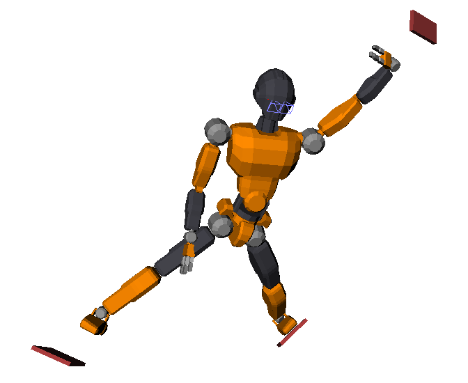
In practice, we can set implicit priorities between tasks by having e.g. $\def\bfA{\boldsymbol{A}} \def\bfB{\boldsymbol{B}} \def\bfC{\boldsymbol{C}} \def\bfD{\boldsymbol{D}} \def\bfE{\boldsymbol{E}} \def\bfF{\boldsymbol{F}} \def\bfG{\boldsymbol{G}} \def\bfH{\boldsymbol{H}} \def\bfI{\boldsymbol{I}} \def\bfJ{\boldsymbol{J}} \def\bfK{\boldsymbol{K}} \def\bfL{\boldsymbol{L}} \def\bfM{\boldsymbol{M}} \def\bfN{\boldsymbol{N}} \def\bfO{\boldsymbol{O}} \def\bfP{\boldsymbol{P}} \def\bfQ{\boldsymbol{Q}} \def\bfR{\boldsymbol{R}} \def\bfS{\boldsymbol{S}} \def\bfT{\boldsymbol{T}} \def\bfU{\boldsymbol{U}} \def\bfV{\boldsymbol{V}} \def\bfW{\boldsymbol{W}} \def\bfX{\boldsymbol{X}} \def\bfY{\boldsymbol{Y}} \def\bfZ{\boldsymbol{Z}} \def\bfalpha{\boldsymbol{\alpha}} \def\bfa{\boldsymbol{a}} \def\bfbeta{\boldsymbol{\beta}} \def\bfb{\boldsymbol{b}} \def\bfcd{\dot{\bfc}} \def\bfchi{\boldsymbol{\chi}} \def\bfc{\boldsymbol{c}} \def\bfd{\boldsymbol{d}} \def\bfe{\boldsymbol{e}} \def\bff{\boldsymbol{f}} \def\bfgamma{\boldsymbol{\gamma}} \def\bfg{\boldsymbol{g}} \def\bfh{\boldsymbol{h}} \def\bfi{\boldsymbol{i}} \def\bfj{\boldsymbol{j}} \def\bfk{\boldsymbol{k}} \def\bflambda{\boldsymbol{\lambda}} \def\bfl{\boldsymbol{l}} \def\bfm{\boldsymbol{m}} \def\bfn{\boldsymbol{n}} \def\bfomega{\boldsymbol{\omega}} \def\bfone{\boldsymbol{1}} \def\bfo{\boldsymbol{o}} \def\bfpdd{\ddot{\bfp}} \def\bfpd{\dot{\bfp}} \def\bfphi{\boldsymbol{\phi}} \def\bfp{\boldsymbol{p}} \def\bfq{\boldsymbol{q}} \def\bfr{\boldsymbol{r}} \def\bfsigma{\boldsymbol{\sigma}} \def\bfs{\boldsymbol{s}} \def\bftau{\boldsymbol{\tau}} \def\bftheta{\boldsymbol{\theta}} \def\bft{\boldsymbol{t}} \def\bfu{\boldsymbol{u}} \def\bfv{\boldsymbol{v}} \def\bfw{\boldsymbol{w}} \def\bfxi{\boldsymbol{\xi}} \def\bfx{\boldsymbol{x}} \def\bfy{\boldsymbol{y}} \def\bfzero{\boldsymbol{0}} \def\bfz{\boldsymbol{z}} \def\defeq{\stackrel{\mathrm{def}}{=}} \def\p{\boldsymbol{p}} \def\qdd{\ddot{\bfq}} \def\qd{\dot{\bfq}} \def\q{\boldsymbol{q}} \def\xd{\dot{x}} \def\yd{\dot{y}} \def\zd{\dot{z}} w_i = 10^4$ for the most important task, $\def\bfA{\boldsymbol{A}} \def\bfB{\boldsymbol{B}} \def\bfC{\boldsymbol{C}} \def\bfD{\boldsymbol{D}} \def\bfE{\boldsymbol{E}} \def\bfF{\boldsymbol{F}} \def\bfG{\boldsymbol{G}} \def\bfH{\boldsymbol{H}} \def\bfI{\boldsymbol{I}} \def\bfJ{\boldsymbol{J}} \def\bfK{\boldsymbol{K}} \def\bfL{\boldsymbol{L}} \def\bfM{\boldsymbol{M}} \def\bfN{\boldsymbol{N}} \def\bfO{\boldsymbol{O}} \def\bfP{\boldsymbol{P}} \def\bfQ{\boldsymbol{Q}} \def\bfR{\boldsymbol{R}} \def\bfS{\boldsymbol{S}} \def\bfT{\boldsymbol{T}} \def\bfU{\boldsymbol{U}} \def\bfV{\boldsymbol{V}} \def\bfW{\boldsymbol{W}} \def\bfX{\boldsymbol{X}} \def\bfY{\boldsymbol{Y}} \def\bfZ{\boldsymbol{Z}} \def\bfalpha{\boldsymbol{\alpha}} \def\bfa{\boldsymbol{a}} \def\bfbeta{\boldsymbol{\beta}} \def\bfb{\boldsymbol{b}} \def\bfcd{\dot{\bfc}} \def\bfchi{\boldsymbol{\chi}} \def\bfc{\boldsymbol{c}} \def\bfd{\boldsymbol{d}} \def\bfe{\boldsymbol{e}} \def\bff{\boldsymbol{f}} \def\bfgamma{\boldsymbol{\gamma}} \def\bfg{\boldsymbol{g}} \def\bfh{\boldsymbol{h}} \def\bfi{\boldsymbol{i}} \def\bfj{\boldsymbol{j}} \def\bfk{\boldsymbol{k}} \def\bflambda{\boldsymbol{\lambda}} \def\bfl{\boldsymbol{l}} \def\bfm{\boldsymbol{m}} \def\bfn{\boldsymbol{n}} \def\bfomega{\boldsymbol{\omega}} \def\bfone{\boldsymbol{1}} \def\bfo{\boldsymbol{o}} \def\bfpdd{\ddot{\bfp}} \def\bfpd{\dot{\bfp}} \def\bfphi{\boldsymbol{\phi}} \def\bfp{\boldsymbol{p}} \def\bfq{\boldsymbol{q}} \def\bfr{\boldsymbol{r}} \def\bfsigma{\boldsymbol{\sigma}} \def\bfs{\boldsymbol{s}} \def\bftau{\boldsymbol{\tau}} \def\bftheta{\boldsymbol{\theta}} \def\bft{\boldsymbol{t}} \def\bfu{\boldsymbol{u}} \def\bfv{\boldsymbol{v}} \def\bfw{\boldsymbol{w}} \def\bfxi{\boldsymbol{\xi}} \def\bfx{\boldsymbol{x}} \def\bfy{\boldsymbol{y}} \def\bfzero{\boldsymbol{0}} \def\bfz{\boldsymbol{z}} \def\defeq{\stackrel{\mathrm{def}}{=}} \def\p{\boldsymbol{p}} \def\qdd{\ddot{\bfq}} \def\qd{\dot{\bfq}} \def\q{\boldsymbol{q}} \def\xd{\dot{x}} \def\yd{\dot{y}} \def\zd{\dot{z}} w_i = 10^2$ for the next one, etc. This is for instance how the pymanoid IK is used in this paper. This solution emulates the behavior of a hierarchical quadratic program (HQP) (unfortunately, there has been no open source HQP solver available as of 2016–2021). See this talk by Wieber (2015) for an deeper overview of the question.

Inequality constraints¶

Last but not least, we need to enforce a number of inequality constraints to avoid solutions that violate e.g. joint limits. The overall IK problem becomes:

Inequalities between vectors being taken componentwise. This time, the pseudo-inverse solution cannot be applied (as it doesn’t handle inequalities), but it is still possible to use a QP solver, such as CVXOPT or quadprog in Python. These solvers work on problems with a quadratic cost function and linear inequalities:

The weighted IK problem falls under this framework.

To go further¶

The formulation that we have seen here is implemented in Python in Pink, an inverse kinematics library based on Pinocchio. Pink comes with a number of examples for manipulators, wheeled biped or humanoid robots. It also runs in real-time motion control loops on the Upkie wheeled biped.