Inverse kinematics
Inverse kinematics (IK) is the problem of computing motions (velocities, accelerations) that make the robot achieve a given set of tasks, such as putting a foot on a surface, moving the center of mass (COM) to a target location, etc. If you are not familiar with these concepts, check out this introduction to inverse kinematics.
Tasks
Tasks are the way to specify objectives to the robot model in a human-readable way.
-
class
pymanoid.tasks.AxisAngleContactTask(robot, link, target, weight=None, gain=None, exclude_dofs=None)¶ Contact task using angle-axis rather than quaternion computations. The benefit of this task is that some degrees of constraint (DOC) of the contact constraint can be (fully or partially) disabled via the doc_mask attribute.
- Parameters
robot (Robot) – Target robot.
link (Link or string) – Robot Link, or name of the link field in the
robotargument.target (list or array (shape=(7,)) or pymanoid.Body) – Pose coordinates of the link’s target.
weight (scalar, optional) – Task weight used in IK cost function. If None, needs to be set later.
gain (scalar, optional) – Proportional gain of the task.
exclude_dofs (list of integers, optional) – DOF indices not used by task.
-
doc_mask¶ Array of dimension six whose values lie between 0 (degree of constraint fully disabled) and 1 (fully enabled). The first three values correspond to translation (Tx, Ty, Tz) while the last three values correspond to rotation (Rx, Ry, Rz).
- Type
array
-
class
pymanoid.tasks.COMAccelTask(robot, weight=None, gain=None, exclude_dofs=None)¶ COM acceleration task.
- Parameters
robot (Humanoid) – Target robot.
target (list or array or Point) – Coordinates or the target COM position.
weight (scalar, optional) – Task weight used in IK cost function. If None, needs to be set later.
gain (scalar, optional) – Proportional gain of the task.
exclude_dofs (list of integers, optional) – DOF indices not used by task.
Notes
Expanding \(\ddot{x}_G = u\) in terms of COM Jacobian and Hessian, the equation of the task is:
\[J_\mathrm{COM} \dot{q}_\mathrm{next} = \frac12 u + J_\mathrm{COM} \dot{q} - \frac12 \delta t \dot{q}^T H_\mathrm{COM} \dot{q}\]See the documentation of the PendulumModeTask for a detailed derivation.
-
class
pymanoid.tasks.COMTask(robot, target, weight=None, gain=None, exclude_dofs=None)¶ COM tracking task.
- Parameters
robot (Humanoid) – Target robot.
target (list or array or Point) – Coordinates or the target COM position.
weight (scalar, optional) – Task weight used in IK cost function. If None, needs to be set later.
gain (scalar, optional) – Proportional gain of the task.
exclude_dofs (list of integers, optional) – DOF indices not used by task.
-
class
pymanoid.tasks.ContactTask(robot, link, target, weight=None, gain=None, exclude_dofs=None)¶ In essence, a contact task is a
pymanoid.tasks.PoseTaskwith a much (much) larger weight. For plausible motions, no task should have a weight higher than (or even comparable to) that of contact tasks.
-
class
pymanoid.tasks.DOFTask(robot, index, target, weight=None, gain=None, exclude_dofs=None)¶ Track a reference DOF value.
- Parameters
robot (Robot) – Target robot.
index (string or integer) – DOF index or string of DOF identifier.
target (scalar) – Target DOF value.
weight (scalar, optional) – Task weight used in IK cost function. If None, needs to be set later.
gain (scalar, optional) – Proportional gain of the task.
exclude_dofs (list of integers, optional) – DOF indices not used by task.
-
class
pymanoid.tasks.MinAccelTask(robot, weight=None, gain=None, exclude_dofs=None)¶ Task to minimize joint accelerations.
- Parameters
robot (Robot) – Target robot.
weight (scalar, optional) – Task weight used in IK cost function. If None, needs to be set later.
gain (scalar, optional) – Gain of the task.
exclude_dofs (list of integers, optional) – DOF indices not used by task.
Note
As the differential IK returns velocities, we approximate the minimization over \(\ddot{q}\) by that over \((\dot{q}_\mathrm{next} - \dot{q})\). See the documentation of the PendulumModeTask for details on the discrete approximation of \(\ddot{q}\).
-
class
pymanoid.tasks.MinCAMTask(robot, weight=None, gain=None, exclude_dofs=None)¶ Minimize the centroidal angular momentum (not its derivative).
- Parameters
robot (Humanoid) – Target robot.
weight (scalar, optional) – Task weight used in IK cost function. If None, needs to be set later.
gain (scalar, optional) – Proportional gain of the task.
exclude_dofs (list of integers, optional) – DOF indices not used by task.
-
class
pymanoid.tasks.MinVelTask(robot, weight=None, gain=None, exclude_dofs=None)¶ Task to minimize joint velocities
- Parameters
robot (Robot) – Target robot.
weight (scalar, optional) – Task weight used in IK cost function. If None, needs to be set later.
gain (scalar, optional) – Proportional gain of the task.
exclude_dofs (list of integers, optional) – DOF indices not used by task.
-
class
pymanoid.tasks.PendulumModeTask(robot, weight=None, gain=None, exclude_dofs=None)¶ Task to minimize the rate of change of the centroidal angular momentum.
- Parameters
robot (Humanoid) – Target robot.
weight (scalar, optional) – Task weight used in IK cost function. If None, needs to be set later.
gain (scalar, optional) – Proportional gain of the task.
exclude_dofs (list of integers, optional) – DOF indices not used by task.
Notes
The way this task is implemented may be surprising. Basically, keeping a constant CAM \(L_G\) means that \(\dot{L}_G = 0\), that is,
\[\frac{\mathrm{d} (J_\mathrm{CAM} \dot{q})}{\mathrm{d} t} = 0 \ \Leftrightarrow\ J_\mathrm{CAM} \ddot{q} + \dot{q}^T H_\mathrm{CAM} \dot{q} = 0\]Because the IK works at the velocity level, we approximate \(\ddot{q}\) by finite difference from the previous robot velocity. Assuming that the velocity \(\dot{q}_\mathrm{next}\) output by the IK is applied immediately, joint angles become:
\[q' = q + \dot{q}_\mathrm{next} \delta t\]Meanwhile, the Taylor expansion of q is
\[q' = q + \dot{q} \delta t + \frac12 \ddot{q} \delta t^2,\]so that applying \(\dot{q}_\mathrm{next}\) is equivalent to having the following constant acceleration over \(\delta t\):
\[\ddot{q} = 2 \frac{\dot{q}_\mathrm{next} - \dot{q}}{\delta t}.\]Replacing in the Jacobian/Hessian expansion yields:
\[2 J_\mathrm{CAM} \frac{\dot{q}_\mathrm{next} - \dot{q}}{\delta t} + + \dot{q}^T H_\mathrm{CAM} \dot{q} = 0.\]Finally, the task in \(\dot{q}_\mathrm{next}\) is:
\[J_\mathrm{CAM} \dot{q}_\mathrm{next} = J_\mathrm{CAM} \dot{q} - \frac12 \delta t \dot{q}^T H_\mathrm{CAM} \dot{q}\]Note how there are two occurrences of \(J_\mathrm{CAM}\): one in the task residual, and the second in the task Jacobian.
-
class
pymanoid.tasks.PosTask(robot, link, target, weight=None, gain=None, exclude_dofs=None)¶ Position task for a given link.
- Parameters
robot (Robot) – Target robot.
link (Link) – One of the Link objects in the kinematic chain of the robot.
target (list or array (shape=(3,)) or pymanoid.Body) – Coordinates of the link’s target.
weight (scalar, optional) – Task weight used in IK cost function. If None, needs to be set later.
gain (scalar, optional) – Proportional gain of the task.
exclude_dofs (list of integers, optional) – DOF indices not used by task.
-
class
pymanoid.tasks.PoseTask(robot, link, target, weight=None, gain=None, exclude_dofs=None)¶ Pose task for a given link.
- Parameters
robot (Robot) – Target robot.
link (Link or string) – Robot Link, or name of the link field in the
robotargument.target (list or array (shape=(7,)) or pymanoid.Body) – Pose coordinates of the link’s target.
weight (scalar, optional) – Task weight used in IK cost function. If None, needs to be set later.
gain (scalar, optional) – Proportional gain of the task.
exclude_dofs (list of integers, optional) – DOF indices not used by task.
-
class
pymanoid.tasks.PostureTask(robot, q_ref, weight=None, gain=None, exclude_dofs=None)¶ Track a set of reference joint angles, a common choice to regularize the weighted IK problem.
- Parameters
robot (Robot) – Target robot.
q_ref (array) – Vector of reference joint angles.
weight (scalar, optional) – Task weight used in IK cost function. If None, needs to be set later.
gain (scalar, optional) – Proportional gain of the task.
exclude_dofs (list of integers, optional) – DOF indices not used by task.
-
class
pymanoid.tasks.Task(weight=None, gain=None, exclude_dofs=None)¶ Generic IK task.
- Parameters
weight (scalar, optional) – Task weight used in IK cost function. If None, needs to be set later.
gain (scalar, optional) – Proportional gain of the task.
exclude_dofs (list of integers, optional) – DOF indices not used by task.
Note
See this tutorial on inverse kinematics for an introduction to the concepts used here.
-
cost(dt)¶ Compute the weighted norm of the task residual.
- Parameters
dt (scalar) – Time step in [s].
- Returns
cost – Current cost value.
- Return type
scalar
-
exclude_dofs(dofs)¶ Exclude additional DOFs from being used by the task.
-
jacobian()¶ Compute the Jacobian matrix of the task.
- Returns
J – Jacobian matrix of the task.
- Return type
array
-
residual(dt)¶ Compute the residual of the task.
- Returns
r – Residual vector of the task.
- Return type
array
Notes
Residuals returned by the
residualfunction must have the unit of a velocity. For instance, \(\dot{q}\) and \((q_1 - q_2) / dt\) are valid residuals, but \(\frac12 q\) is not.
Solver
The IK solver is the numerical optimization program that converts task targets and the current robot state to joint motions. In pymanoid, joint motions are computed as velocities that are integrated forward during each simulation cycle (other IK solvers may compute acceleration or jerk values, which are then integrated twice or thrice respectively).
-
class
pymanoid.ik.IKSolver(robot, active_dofs=None, doflim_gain=0.5)¶ Compute velocities bringing the system closer to fulfilling a set of tasks.
- Parameters
robot (Robot) – Robot to be updated.
active_dofs (list of integers, optional) – List of DOFs updated by the IK solver.
doflim_gain (scalar, optional) – DOF-limit gain as described in [Kanoun12]. In this implementation, it should be between zero and one.
-
doflim_gain¶ DOF-limit gain as described in [Kanoun12]. In this implementation, it should be between zero and one.
- Type
scalar, optional
-
lm_damping¶ Add Levenberg-Marquardt damping as described in [Sugihara11]. This damping significantly improves numerical stability, but convergence gets slower when its value is too high.
- Type
scalar
-
slack_dof_limits¶ Add slack variables to maximize DOF range? This method is used in [Nozawa16] to keep joint angles as far away from their limits as possible. It slows down computations as there are twice as many optimization variables, but is more numerically stable and won’t produce inconsistent constraints. Defaults to False.
- Type
bool
-
slack_maximize¶ Linear cost weight applied when
slack_dof_limitsis True.- Type
scalar
-
slack_regularize¶ Regularization weight applied when
slack_dof_limitsis True.- Type
scalar
-
qd¶ Velocity returned by last solver call.
- Type
array
-
robot¶ Robot model.
- Type
pymanoid.Robot
-
tasks¶ Dictionary of active IK tasks, indexed by task name.
- Type
dict
Notes
One unsatisfactory aspect of the DOF-limit gain is that it slows down the robot when approaching DOF limits. For instance, it may slow down a foot motion when approaching the knee singularity, despite the robot being able to move faster with a fully extended knee.
-
build_qp_matrices(dt)¶ Build matrices of the quatratic program.
- Parameters
dt (scalar) – Time step in [s].
- Returns
P ((n, n) array) – Positive semi-definite cost matrix.
q (array) – Cost vector.
qd_max (array) – Maximum joint velocity vector.
qd_min (array) – Minimum joint velocity vector.
Notes
When the robot model has joint acceleration limits, special care should be taken when computing the corresponding velocity bounds for the IK. In short, the robot now needs to avoid the velocity range where it (1) is not going to collide with a DOF limit in one iteration but (2) cannot brake fast enough to avoid a collision in the future due to acceleration limits. This function implements the solution to this problem described in Equation (14) of [Flacco15].
-
clear()¶ Clear all tasks in the IK solver.
-
compute_cost(dt)¶ Compute the IK cost of the present system state for a time step of dt.
- Parameters
dt (scalar) – Time step in [s].
-
compute_velocity(dt)¶ Compute a new velocity satisfying all tasks at best.
- Parameters
dt (scalar) – Time step in [s].
- Returns
qd – Vector of active joint velocities.
- Return type
array
Note
This QP formulation is the default for
pymanoid.ik.IKSolver.solve()(posture generation) as it converges faster.Notes
The method implemented in this function is reasonably fast but may become unstable when some tasks are widely infeasible. In such situations, you can either increase the Levenberg-Marquardt bias
self.lm_dampingor setslack_dof_limits=Truewhich will callpymanoid.ik.IKSolver.compute_velocity_with_slack().The returned velocity minimizes squared residuals as in the weighted cost function, which corresponds to the Gauss-Newton algorithm. Indeed, expanding the square expression in
cost(task, qd)yields\[\mathrm{minimize} \ \dot{q} J^T J \dot{q} - 2 r^T J \dot{q}\]Differentiating with respect to \(\dot{q}\) shows that the minimum is attained for \(J^T J \dot{q} = r\), where we recognize the Gauss-Newton update rule.
-
compute_velocity_with_slack(dt)¶ Compute a new velocity satisfying all tasks at best, while trying to stay away from kinematic constraints.
- Parameters
dt (scalar) – Time step in [s].
- Returns
qd – Vector of active joint velocities.
- Return type
array
Note
This QP formulation is the default for
pymanoid.ik.IKSolver.step()as it has a more numerically-stable behavior.Notes
Check out the discussion of this method around Equation (10) of [Nozawa16]. DOF limits are better taken care of by slack variables, but the variable count doubles and the QP takes roughly 50% more time to solve.
-
on_tick(sim)¶ Step the IK at each simulation tick.
- Parameters
sim (Simulation) – Simulation instance.
-
print_costs(qd, dt)¶ Print task costs for the current IK step.
- Parameters
qd (array) – Robot DOF velocities.
dt (scalar) – Timestep for the IK.
-
remove(ident)¶ Remove a task.
- Parameters
ident (string or object) – Name or object with a
namefield identifying the task.
-
set_active_dofs(active_dofs)¶ Set DOF indices modified by the IK.
- Parameters
active_dofs (list of integers) – List of DOF indices.
-
set_gains(gains)¶ Set task gains from a dictionary.
- Parameters
gains (string -> double dictionary) – Dictionary mapping task labels to default gain values.
-
set_weights(weights)¶ Set task weights from a dictionary.
- Parameters
weights (string -> double dictionary) – Dictionary mapping task labels to default weight values.
-
solve(max_it=1000, cost_stop=1e-10, impr_stop=1e-05, dt=0.01, warm_start=False, debug=False)¶ Compute joint-angles that satisfy all kinematic constraints at best.
- Parameters
max_it (integer) – Maximum number of solver iterations.
cost_stop (scalar) – Stop when cost value is below this threshold.
impr_stop (scalar, optional) – Stop when cost improvement (relative variation from one iteration to the next) is less than this threshold.
dt (scalar, optional) – Time step in [s].
warm_start (bool, optional) – Set to True if the current robot posture is a good guess for IK. Otherwise, the solver will start by an exploration phase with DOF velocity limits relaxed and no Levenberg-Marquardt damping.
debug (bool, optional) – Set to True for additional debug messages.
- Returns
nb_it (int) – Number of solver iterations.
cost (scalar) – Final value of the cost function.
Notes
Good values of dt depend on the weights of the IK tasks. Small values make convergence slower, while big values make the optimization unstable (in which case there may be no convergence at all).
-
step(dt)¶ Apply velocities computed by inverse kinematics.
- Parameters
dt (scalar) – Time step in [s].
Acceleration limits
When the robot model has joint acceleration limits, i.e. when a vector of
size robot.nb_dofs is specified in robot.qdd_lim at initialization, the
inverse kinematics will include them in its optimization problem. The
formulation is more complex than a finite-difference approximation: joint
velocities will be selected so that (1) the joint does not collide with its
position limit in one iteration, but also (2) despite its acceleration limit,
it can still brake fast enough to avoid colliding with its position limit in
the future. The inverse kinematics in pymanoid implements the solution to this
problem described in Equation (14) of [Flacco15].
Stance
The most common IK tasks for humanoid locomotion are the COM task and end-effector pose task. The Stance class avoids the hassle of
creating and adding these tasks one by one. To use it, first create your targets:
com_target = robot.get_com_point_mass()
lf_target = robot.left_foot.get_contact(pos=[0, 0.3, 0])
rf_target = robot.right_foot.get_contact(pos=[0, -0.3, 0])
Then create the stance and bind it to the robot:
stance = Stance(com=com_target, left_foot=lf_target, right_foot=rf_target)
stance.bind(robot)
Calling the bind function will automatically add the corresponding tasks to the robot IK solver. See the inverse_kinematics.py example for more details.
-
class
pymanoid.stance.Stance(com, left_foot=None, right_foot=None, left_hand=None, right_hand=None)¶ Set of contact and center of mass (COM) targets for the humanoid.
- Parameters
com (PointMass) – Center of mass target.
left_foot (Contact, optional) – Left-foot contact target.
right_foot (Contact, optional) – Right-foot contact target.
left_hand (Contact, optional) – Left-hand contact target.
right_hand (Contact, optional) – Right-hand contact target.
-
bind(robot, reg='posture')¶ Bind stance as robot IK targets.
- Parameters
robot (pymanoid.Robot) – Target robot.
reg (string, optional) – Regularization task, either “posture” or “min_vel”.
-
property
bodies¶ List of end-effector and COM bodies.
-
compute_pendular_accel_cone(com_vertices=None, zdd_max=None, reduced=False)¶ Compute the pendular COM acceleration cone of the stance.
The pendular cone is the reduction of the Contact Wrench Cone when the angular momentum at the COM is zero.
- Parameters
com_vertices (list of (3,) arrays, optional) – Vertices of a COM bounding polytope.
zdd_max (scalar, optional) – Maximum vertical acceleration in the output cone.
reduced (bool, optional) – If
True, returns the reduced 2D form rather than a 3D cone.
- Returns
vertices – List of 3D vertices of the (truncated) COM acceleration cone, or of the 2D vertices of the reduced form if
reducedisTrue.- Return type
list of (3,) arrays
Notes
The method is based on a rewriting of the CWC formula, followed by a 2D convex hull on dual vertices. The algorithm is described in [Caron16].
When
comis a list of vertices, the returned cone corresponds to COM accelerations that are feasible from all COM located inside the polytope. See [Caron16] for details on this conservative criterion.
-
compute_static_equilibrium_polygon(method='hull')¶ Compute the halfspace and vertex representations of the static-equilibrium polygon (SEP) of the stance.
- Parameters
method (string, optional) – Which method to use to perform the projection. Choices are ‘bretl’, ‘cdd’ and ‘hull’ (default).
-
compute_zmp_support_area(height, method='bretl')¶ Compute an extension of the (pendular) multi-contact ZMP support area with optional pressure limits on each contact.
- Parameters
height (array, shape=(3,)) – Height at which the ZMP support area is computed.
method (string, default='bretl') – Polytope projection algorithm, can be
"bretl"or"cdd".
- Returns
vertices – Vertices of the ZMP support area.
- Return type
list of arrays
Notes
There are two polytope projection algorithms: ‘bretl’ is adapted from in [Bretl08] while ‘cdd’ corresponds to the double-description formulation from [Caron17z]. See the Appendix from [Caron16] for a performance comparison.
-
property
contacts¶ List of active contacts.
-
dist_to_sep_edge(com)¶ Algebraic distance of a COM position to the edge of the static-equilibrium polygon.
- Parameters
com (array, shape=(3,)) – COM position to evaluate the distance from.
- Returns
dist – Algebraic distance to the edge of the polygon. Inner points get a positive value, outer points a negative one.
- Return type
scalar
-
find_static_supporting_wrenches()¶ Find supporting contact wrenches in static-equilibrium.
- Returns
support – Mapping between each contact i in the contact set and a supporting contact wrench \(w^i_{C_i}\).
- Return type
list of (Contact, array) couples
-
free_contact(effector_name)¶ Free a contact from the stance and get the corresponding end-effector target. Its task stays in the IK, but the effector is not considered in contact any more (e.g. for contact wrench computations).
- Parameters
effector_name (string) – Name of end-effector target, for example “left_foot”.
- Returns
effector – IK target contact.
- Return type
pymanoid.Contact
-
static
from_json(path)¶ Create a new stance from a JSON file.
- Parameters
path (string) – Path to the JSON file.
-
hide()¶ Hide end-effector and COM body handles.
-
load(path)¶ Load stance from JSON file.
- Parameters
path (string) – Path to the JSON file.
-
property
nb_contacts¶ Number of active contacts.
-
save(path)¶ Save stance into JSON file.
- Parameters
path (string) – Path to JSON file.
-
set_contact(effector)¶ Set contact on a effector.
- Parameters
effector (pymanoid.Contact) – IK target contact.
-
show()¶ Show end-effector and COM body handles.
Example
In this example, we will see how to put the humanoid robot model in a desired configuration. Let us initialize a simulation with a 30 ms timestep and load the JVRC-1 humanoid:
sim = pymanoid.Simulation(dt=0.03)
robot = JVRC1('JVRC-1.dae', download_if_needed=True)
sim.set_viewer()  # open GUI window
We define targets for foot contacts;
lf_target = Contact(robot.sole_shape, pos=[0, 0.3, 0], visible=True)
rf_target = Contact(robot.sole_shape, pos=[0, -0.3, 0], visible=True)
Next, let us set the altitude of the robot’s free-flyer (attached to the waist link) 80 cm above contacts. This is useful to give the IK solver a good initial guess and avoid coming out with a valid but weird solution in the end.
robot.set_dof_values([0.8], dof_indices=[robot.TRANS_Z])
This being done, we initialize a point-mass that will serve as center-of-mass
(COM) target for the IK. Its initial position is set to robot.com, which
will be roughly 80 cm above contacts as it is close to the waist link:
com_target = PointMass(pos=robot.com, mass=robot.mass)
All our targets being defined, we initialize IK tasks for the feet and COM position, as well as a posture task for the (necessary) regularization of the underlying QP problem:
lf_task = ContactTask(robot, robot.left_foot, lf_target, weight=1.)
rf_task = ContactTask(robot, robot.right_foot, rf_target, weight=1.)
com_task = COMTask(robot, com_target, weight=1e-2)
reg_task = PostureTask(robot, robot.q, weight=1e-6)
We initialize the robot’s IK using all DOFs, and insert our tasks:
robot.init_ik(active_dofs=robot.whole_body)
robot.ik.add_task(lf_task)
robot.ik.add_task(rf_task)
robot.ik.add_task(com_task)
robot.ik.add_task(reg_task)
We can also throw in some extra DOF tasks for a nicer posture:
robot.ik.add_task(DOFTask(robot, robot.R_SHOULDER_R, -0.5, gain=0.5, weight=1e-5))
robot.ik.add_task(DOFTask(robot, robot.L_SHOULDER_R, +0.5, gain=0.5, weight=1e-5))
Finally, call the IK solver to update the robot posture:
robot.ik.solve(max_it=100, impr_stop=1e-4)
The resulting posture looks like this:
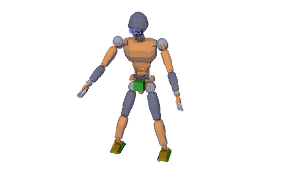
Robot posture found by inverse kinematics.
Alternatively, rather than creating and adding all tasks one by one, we could have used the Stance interface:
stance = Stance(com=com_target, left_foot=lf_target, right_foot=rf_target)
stance.bind(robot)
robot.ik.add_task(DOFTask(robot, robot.R_SHOULDER_R, -0.5, gain=0.5, weight=1e-5))
robot.ik.add_task(DOFTask(robot, robot.L_SHOULDER_R, +0.5, gain=0.5, weight=1e-5))
robot.ik.solve(max_it=100, impr_stop=1e-4)
This code is more concise and yields the same result.