Walking pattern generation
Walking pattern generation converts a high-level objective such as “go through this sequence of footsteps” to a time-continuous joint trajectory. For position-controlled robots such as those simulated in pymanoid, joint trajectories are computed by inverse kinematics from intermediate task targets. The two main targets for walking are the swing foot and center of mass.
Swing foot trajectory
The foot in the air during a single-support phase is called the swing foot. Its trajectory can be implemented by spherical linear interpolation for the orientation and polynomial interpolation for the position of the foot in the air.
-
class
pymanoid.swing_foot.SwingFoot(start_contact, end_contact, duration, takeoff_clearance=0.05, landing_clearance=0.05)¶ Polynomial swing foot interpolator.
- Parameters
start_contact (pymanoid.Contact) – Initial contact.
end_contact (pymanoid.Contact) – Target contact.
duration (scalar) – Swing duration in [s].
takeoff_clearance (scalar, optional) – Takeoff clearance height at 1/4th of the interpolated trajectory.
landing_clearance (scalar, optional) – Landing clearance height at 3/4th of the interpolated trajectory.
-
draw(color='r')¶ Draw swing foot trajectory.
- Parameters
color (char or triplet, optional) – Color letter or RGB values, default is ‘b’ for blue.
-
integrate(dt)¶ Integrate swing foot motion forward by a given amount of time.
- Parameters
dt (scalar) – Duration of forward integration, in [s].
-
interpolate()¶ Interpolate swing foot path.
- Returns
path – Polynomial path with index between 0 and 1.
- Return type
pymanoid.NDPolynomial
Notes
A swing foot trajectory comes under two conflicting imperatives: stay close to the ground while avoiding collisions. We assume here that the terrain is uneven but free from obstacles. To avoid robot-ground collisions, we enforce two clearance distances: one at toe level for the takeoff contact and the other at heel level for the landing contact.
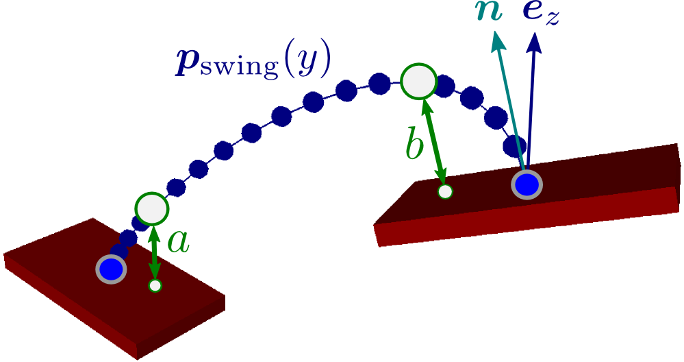
We interpolate swing foot trajectories as cubic Hermite curves with four boundary constraints: initial and final positions corresponding to contact centers, and tangent directions parallel to contact normals. This leaves two free parameters, corresponding to the norms of the initial and final tangents, that can be optimized upon. It can be shown that minimizing these two parameters subject to the clearance conditions
a > a_minandb > b_minis a small constrained least squares problem.
Linear model predictive control
Linear model predictive control [Wieber06] generates a dynamically-consistent trajectory for the center of mass (COM) while walking. It applies to walking over a flat floor, where the assumptions of the linear inverted pendulum mode (LIPM) [Kajita01] can be applied.
-
class
pymanoid.mpc.LinearPredictiveControl(A, B, C, D, e, x_init, x_goal, nb_steps, wxt=None, wxc=None, wu=0.001)¶ Predictive control for a system with linear dynamics and linear constraints.
The discretized dynamics of a linear system are described by:
\[x_{k+1} = A x_k + B u_k\]where \(x\) is assumed to be the first-order state of a configuration variable \(p\), i.e., it stacks both the position \(p\) and its time-derivative \(\dot{p}\). Meanwhile, the system is linearly constrained by:
\[\begin{split}x_0 & = x_\mathrm{init} \\ \forall k, \ C_k x_k + D_k u_k & \leq e_k \\\end{split}\]The output control law minimizes a weighted combination of two types of costs:
- Terminal state error
\(\|x_\mathrm{nb\_steps} - x_\mathrm{goal}\|^2\) with weight \(w_{xt}\).
- Cumulated state error:
\(\sum_k \|x_k - x_\mathrm{goal}\|^2\) with weight \(w_{xc}\).
- Cumulated control costs:
\(\sum_k \|u_k\|^2\) with weight \(w_{u}\).
- Parameters
A (array, shape=(n, n)) – State linear dynamics matrix.
B (array, shape=(n, dim(u))) – Control linear dynamics matrix.
x_init (array, shape=(n,)) – Initial state as stacked position and velocity.
x_goal (array, shape=(n,)) – Goal state as stacked position and velocity.
nb_steps (int) – Number of discretization steps in the preview window.
C (array, shape=(m, dim(u)), list of arrays, or None) – Constraint matrix on state variables. When this argument is an array, the same matrix C is applied at each step k. When it is
None, the null matrix is applied.D (array, shape=(l, n), or list of arrays, or None) – Constraint matrix on control variables. When this argument is an array, the same matrix D is applied at each step k. When it is
None, the null matrix is applied.e (array, shape=(m,), list of arrays) – Constraint vector. When this argument is an array, the same vector e is applied at each step k.
wxt (scalar, optional) – Weight on terminal state cost, or
Noneto disable.wxc (scalar, optional) – Weight on cumulated state costs, or
Noneto disable (default).wu (scalar, optional) – Weight on cumulated control costs.
Notes
In numerical analysis, there are three classes of methods to solve boundary value problems: single shooting, multiple shooting and collocation. The solver implemented in this class follows the single shooting method.
-
property
X¶ Series of system states over the preview window.
Note
This property is only available after
solve()has been called.
-
build()¶ Compute internal matrices defining the preview QP.
Notes
See [Audren14] for details on the matrices \(\Phi\) and \(\Psi\), as we use similar notations below.
-
solve(**kwargs)¶ Compute the series of controls that minimizes the preview QP.
- Parameters
solver (string, optional) – Name of the QP solver in
qpsolvers.available_solvers.initvals (array, optional) – Vector of initial U values used to warm-start the QP solver.
-
property
solve_and_build_time¶ Total computation time taken by MPC computations.
Nonlinear predictive control
The assumptions of the LIPM are usually too restrictive to walk over uneven
terrains. In this case, one can turn to more general (nonlinear) model
predictive control. A building block for nonlinear predictive control of the
center of mass is implemented in the
pymanoid.centroidal.COMStepTransit class, where a COM trajectory is
constructed from one footstep to the next by solving a nonlinear program (NLP).
-
class
pymanoid.centroidal.COMStepTransit(desired_duration, start_com, start_comd, dcm_target, foothold, next_foothold, omega2, nb_steps, nlp_options=None)¶ Compute a COM trajectory that transits from one footstep to the next. This solution is applicable over arbitrary terrains.
Implements a short-sighted optimization with a DCM boundedness constraint, defined within the floating-base inverted pendulum (FIP) of constant \(\omega\). This approach is used in the nonlinear predictive controller of [Caron17w] for dynamic walking over rough terrains.
- Parameters
desired_duration (scalar) – Desired duration of the transit trajectory.
start_com ((3,) array) – Initial COM position.
start_comd ((3,) array) – Initial COM velocity.
foothold (Contact) – Location of the stance foot contact.
omega (scalar) – Constant of the floating-base inverted pendulum.
dcm_target ((3,) array) – Desired terminal divergent-component of COM motion.
nb_steps (int) – Number of discretization steps.
Notes
The boundedness constraint in this optimization makes up for the short-sighted preview [Scianca16], as opposed to the long-sighted approach to walking [Wieber06] where COM boundedness results from the preview of several future steps.
The benefit of using ZMP controls rather than COM accelerations lies in the exact integration scheme. This phenomenon appears in flat-floor models as well: in the CART-table model, segments with fixed COM acceleration imply variable ZMPs that may exit the support area (see e.g. Figure 3.17 in [ElKhoury13]).
-
add_com_height_constraint(p, ref_height, max_dev)¶ Constraint the COM to deviate by at most max_dev from ref_height.
- Parameters
ref_height (scalar) – Reference COM height.
max_dev (scalar) – Maximum distance allowed from the reference.
Note
The height is measured along the z-axis of the contact frame here, not of the world frame’s.
-
add_friction_constraint(p, z, foothold)¶ Add a circular friction cone constraint for a COM located at p and a (floating-base) ZMP located at z.
- Parameters
p (casadi.MX) – Symbol of COM position variable.
z (casadi.MX) – Symbol of ZMP position variable.
-
add_linear_cop_constraints(p, z, foothold, scaling=0.95)¶ Constraint the COP, located between the COM p and the (floating-base) ZMP z, to lie inside the contact area.
- Parameters
p (casadi.MX) – Symbol of COM position variable.
z (casadi.MX) – Symbol of ZMP position variable.
scaling (scalar, optional) – Scaling factor between 0 and 1 applied to the contact area.
-
build()¶ Build the internal nonlinear program (NLP).
-
draw(color='b')¶ Draw the COM trajectory.
- Parameters
color (char or triplet, optional) – Color letter or RGB values, default is ‘b’ for green.
- Returns
handle – OpenRAVE graphical handle. Must be stored in some variable, otherwise the drawn object will vanish instantly.
- Return type
openravepy.GraphHandle
-
print_results()¶ Print various statistics on NLP resolution.
-
solve()¶ Solve the nonlinear program and store the solution, if found.