Perspectives on Motion Planning and Control for Humanoid Robots in Multi-contact Scenarios

Stéphane Caron
Nakamura-Takano Laboratory
Seminar @ NTU
March 7^th, 2016

Motivation

Scope

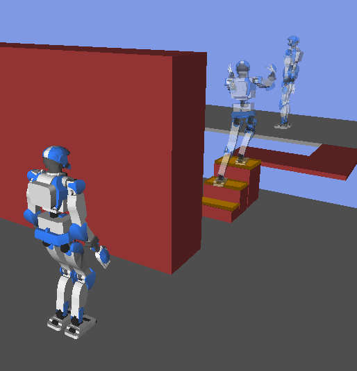
Autonomous planning and execution of motions on a humanoid robot.

Challenges

Perception has low rate update loops
Planning in space and time
Control under kinodynamic constraints:
- Underactuation of world coordinates
- Nonholonomy from angular momentum
- Switching contact dynamics
etc.

The Feedback loop

Ideal model

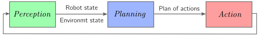
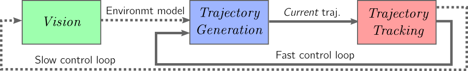
Robots implement the perception-planning-action loop:

State of the art

Current implementations are closer to the following:

The Feedback loop (cont'd)

Enters non-holonomy

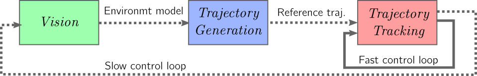
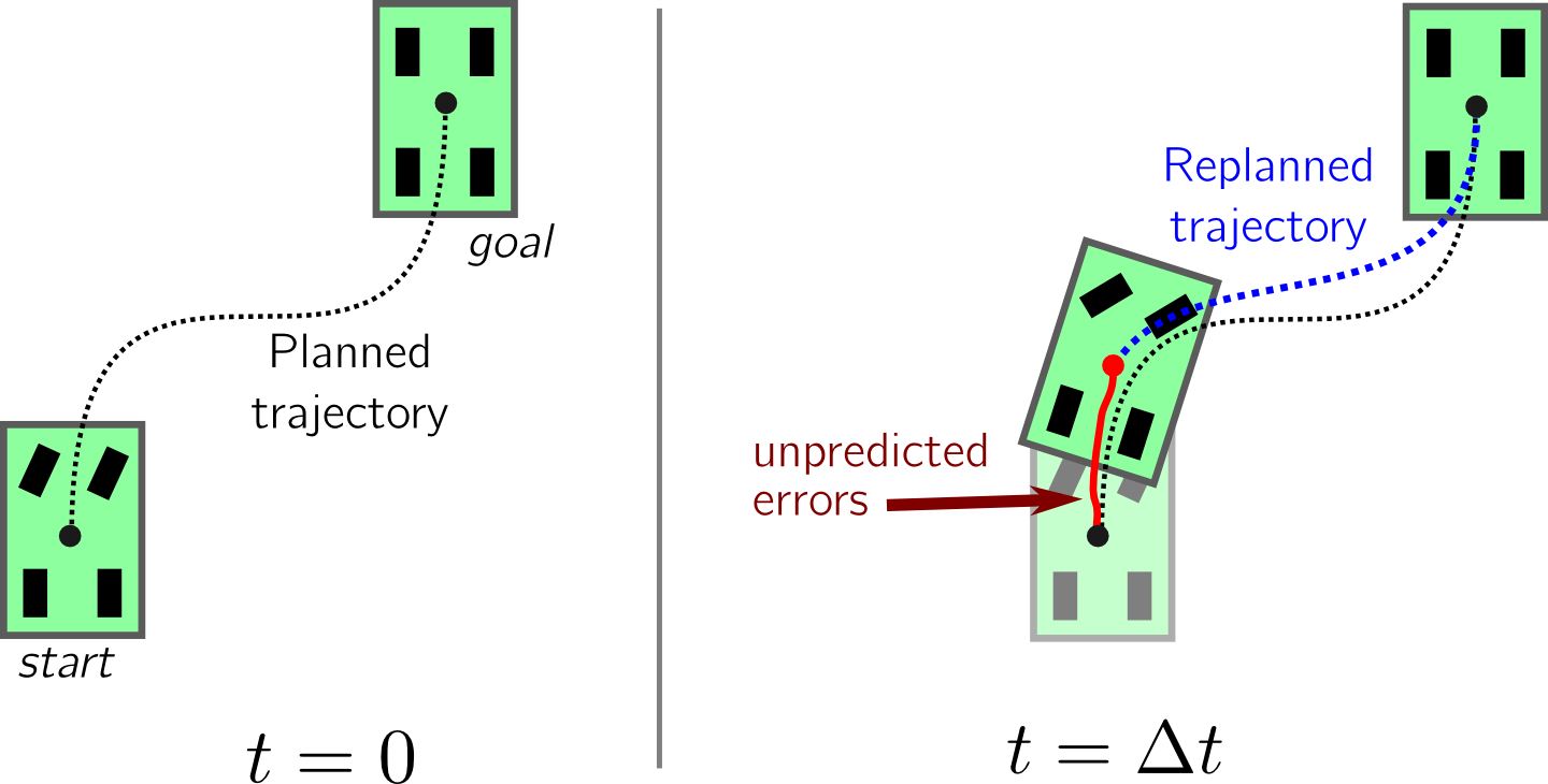
Illustration on a Reeds & Shepp car model.

Assuming good trajectory tracking is a holonomic approximation, but humanoids are subject to a nonholonomic constraint. Nonholonomy can be addressed with a continuous replanner updating the reference trajectory in real time.

Motion Planning

Problem: find a trajectory from the robot's current state to some goal state.

Terminology

$q \in C \subset R^{n}$ : configuration space
$x \in X \subset R^{2 n}$ : state space, positions and velocities
Path: purely geometric: $s \mapsto q (s) \in C$
Trajectory: path and time: $t \mapsto q (s (t))$

Property

Trajectories $t \mapsto q (t)$ in the configuration space $C$ are paths in the state-space $X .$

Kinematic Motion Planning

(Adapted from: Eric O. Scott)

Historically, kinematic systems were considered first. ^{(Latombe, 1991)}

Kinematic constraints
Apply to configurations $q$
Joint limits $\| q \| \leq q_{max}$
Collision avoidance $d_{o b s} (q) > ϵ$
Maintain contacts $f (q) = 0$

Kinematic planning is done in the configuration space $C$ of the robot.

The main challenge is collision avoidance

Roadmap Planners

Idea

Build a roadmap (graph) $G = (V, E)$ over the configuration space $C$ of the robots. Nodes are configurations $V = {q_{1}, q_{2}, \dots}$ and edges represent paths.

Approach

Initialization:
- $G = ({q_{i n i t}}, \emptyset)$
Extension:
- Generate a new node $q^{'} \in C$
- Try to connect $q^{'}$ to some $q \in V$
Termination (optional):
- Try to connect a target $q_{g o a l}$

Stochastic Roadmap Planners

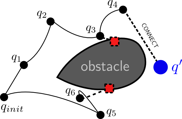
(Source: Eric O. Scott)

A roadmap planner turns a local planner into a global one, enforcing additional constraints such as collision avoidance.

Probabilistic Roadmaps (PRM)

Multiple-query model: grow the roadmap uniformly at random, connect pairs of configurations using graph search and the local planner.^{(Kavraki et al., 1996)}

Rapidly-exploring Random Trees (RRT)

Single-query model: try to connect the initial configuration to the goal as fast as possible.^{(LaValle et al., 1998)}

Completeness

The planner can tell in finite time whether there are solutions, and if so find one.

Probabilistic completeness

If there are solution, the planner will find one given enough computation time:

P (solution found after N extensions) N \to \infty - --- \to 1.

Unless the planner finds a solution, it is impossible to distinguish the cases where (1) more extensions are required, or (2) the problem has no solution.

A correctness guarantee

Completeness proofs formalize the requirements of a motion planner, e.g. full actuation, minimum obstacle clearance, etc.

Completeness of Kinematic Planners

Both PRM and RRT are probabilistically complete for kinematic path planning.

Theorem (Kavraki et al., 1998)

Let $γ : [0, L] \to F$ be a path of (Euclidean) length $L$ , with $γ (0) = a$ , $γ (L) = b$ and let $R = {inf}_{0 \leq t \leq L} r (γ (t))$ be the distance of the path of the obstacles. Then the probability that [PRM] will fail to connect the points $a$ and $b$ is at most $\frac{2 L}{R} (1 - α R^{2})^{N}$ , where $α = π / (4 | F |)$ .

Theorem (LaValle and Kuffner, 2000)

The RRT-Connect algorithm is probabilistically complete and vertices [of the roadmap] converge to a uniform distribution over $C_{f r e e}$ .

Kinodynamic Planning

Dynamic systems are constrained in two ways: ^{(Donald et al., 1993)}

˙ x = f (x, u) \Leftrightarrow M (q) ¨ q + {˙ q}^{⊤} C (q) ˙ q + g (q) = τ + J^{⊤} f

Kinematic constraints	Dynamic constraints
Apply to configurations $q$	Include time-derivatives $˙ q$ and $¨ q$
Joint limits $\| q \| \leq q_{max}$	Velocity limits: $\| ˙ q \| \leq {˙ q}_{max}$
Collision avoidance (self, obstacles)	Torque limits: $\| τ (q, ˙ q, ¨ q) \| \leq τ_{max}$
Maintain contacts (position)	Maintain contacts (friction)

To take all into account, kinodynamic planning is usually done in the state space $X$ , which is by nature more complex than $C$ .

Completeness of Kinodyn. Planners

Yes	No
(LaValle and Kuffner, 2001): RRT is probabilistically complete for kinodynamic planning.	(Kunz and Stilman, 2015): RRT with fixed time step and best-input extension is not prob. complete.
(Hsu et al., 2002): PRM is prob. complete in $(α, β)$ -expansive state spaces when $α > 0$ .	(Hsu et al., 1997): checking if $α > 0$ is as hard as solving the planning problem itself.
(Papadopoulos et al., 2014): RRT with random piecewise-constant controls is probabilistically complete.	(Caron et al., 2014): RRT with fixed time step and Bezier curve interpolation is is not prob. complete.
(Caron et al., 2014): RRT with acceleration-compliant interpolation is probabilistically complete.	Source of the confusion: need to specify both planner and extension functions.

Steering functions

The steering function is the local planner that connects two configurations $x_{1}$ and $x_{2}$ by a trajectory $x : [0, T] \to C$ with $x (0) = x_{1}$ and $x (T) = x_{2}$ .

Analytical steering

A perfect solution can be found mathematically, as e.g. for Reeds and Shepp curves used in non-holonomic planners. ^{(Laumond et al., 1998)}

Control-based steering

Control functions $u (t)$ are sampled and their response simulated by forward dynamics. ^{(LaValle, 2001)} Applies to a wide range of systems, but not humanoids.

State-based steering

A state trajectory $q : [0, T] \to C$ is interpolated, then tracked by inverse dynamics. Commonly used in humanoid motion planning.

Completeness guarantee ^{(ICRA 2014)}

Theorem

Consider a time-invariant differential system with Lipschitz-smooth dynamics $f$ and full actuation. Suppose that the kinodynamic planning problem between two states $x_{i n i t}$ and $x_{g o a l}$ admits a smooth solution $γ : [0, T] \to C$ with $δ$ -clearance in control space. A randomized motion planner using a acceleration-compliant interpolation function is probabilistically complete.

Acceleration compliance

When $x^{'} \to x$ , the interpolation from $x$ to $x^{'}$ stays within a neighborhood of $x$ and its accelerations converges to $\frac{∥ ˙ q ∥ ∥ Δ q ∥}{∥ Δ ˙ q ∥}$ , the discrete acceleration encoded in $Δ x$ .

Comparison in simulations

System

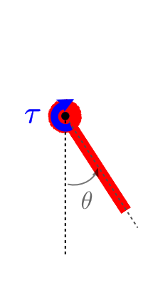
Pendulum with low torques $| τ | \leq 5$ Nm.
Requires multiple swings in order to lift up.

Results

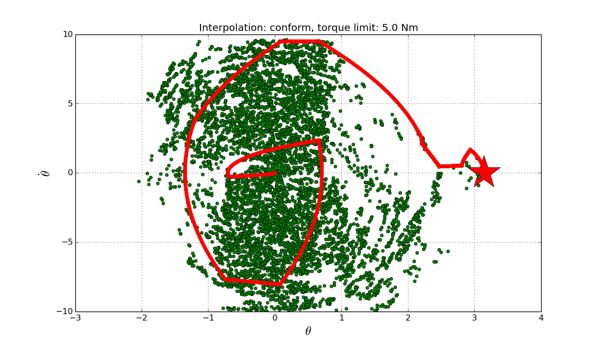Acceleration-compliant interpolation

Bezier curves with fixed time step

State Space

By Jc86035 (Bézier 2 big.png, by Phil Tregoning (Twirlip)) [Public domain], via Wikimedia Commons

Definition

$X := {x = (q, ˙ q), q \in C, ˙ q \in R^{n}}$ .

Structure

The state space $X$ has:

a manifold structure $d q = ˙ q d t$
high dimension $2 n$ (positions and velocities)

Also: never been used for humanoid motion planning.

Interpolation

Acceleration-compliant interpolation functions are not straightforward to find for multi-DOF systems.

Decoupling of the state space

Ideally

Kinematic motion planning in $C$
Dynamic parameterization from $C$ to $X$

Followed e.g. by (Kuffner et al., 2002), yet with limitation to quasi-static trajectories (no dynamic motion).

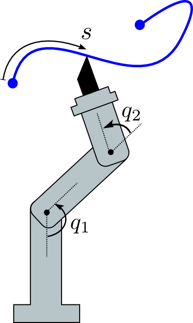
Time-Optimal Path Parameterization (TOPP)

Converts a path $q (s)$ into a feasible trajectory $q (s (t))$ with minimum duration $T$ .

Provides a mapping from $C$ to $X$ paths.
Enforces fully-determined kinodynamic constraints

Direct-integration method proposed in (Bobrow et al., 1985).

Initial limits of TOPP

Switching contact dynamics

How to go through contact switches dynamically, i.e. without stopping at quasi-static configurations.

Integration with motion planning

Retiming after planning is highly inefficient. For example, if the path is dynamically unfeasible 5% of the start, the remaining 95% of path planning computations were unnecessary.

Velocity Propagation ^{(RSS 2013)}

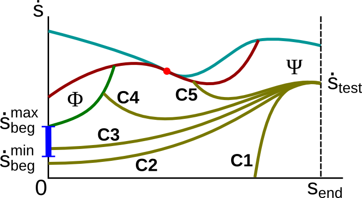
Limiting curves in the phase-space $(s, ˙ s)$ of a path $q (s)$ .

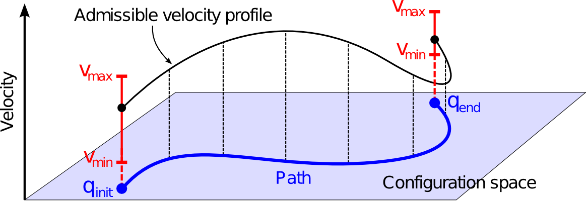
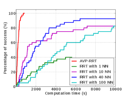
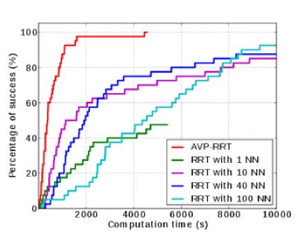
The AVP-RRT planner separates path and velocity planning thanks to AVP.

Admissible Velocity Propagation

We extend existing TOPP methods to find the interval of reachable velocities along a path.

(q (s), [v_{min}, v_{max}]^{i n i t}) A V P - -- \to [v_{min}, v_{max}]^{e n d}

AVP-RRT planner

Integration with a configuration-space RRT where nodes are augmented with velocity intervals $(q, [v_{min}, v_{max}])$ .

Completeness guarantee

AVP-RRT is (almost) probabilistically complete.

Experiments

System

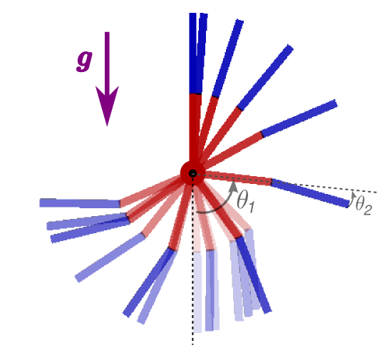
Double-pendulum with low torques.
Requires multiple swings in order to lift up.

Comparison to state-space planners

Torque limit (11, 7) Nm

Torque limit (11, 5) Nm

Friction

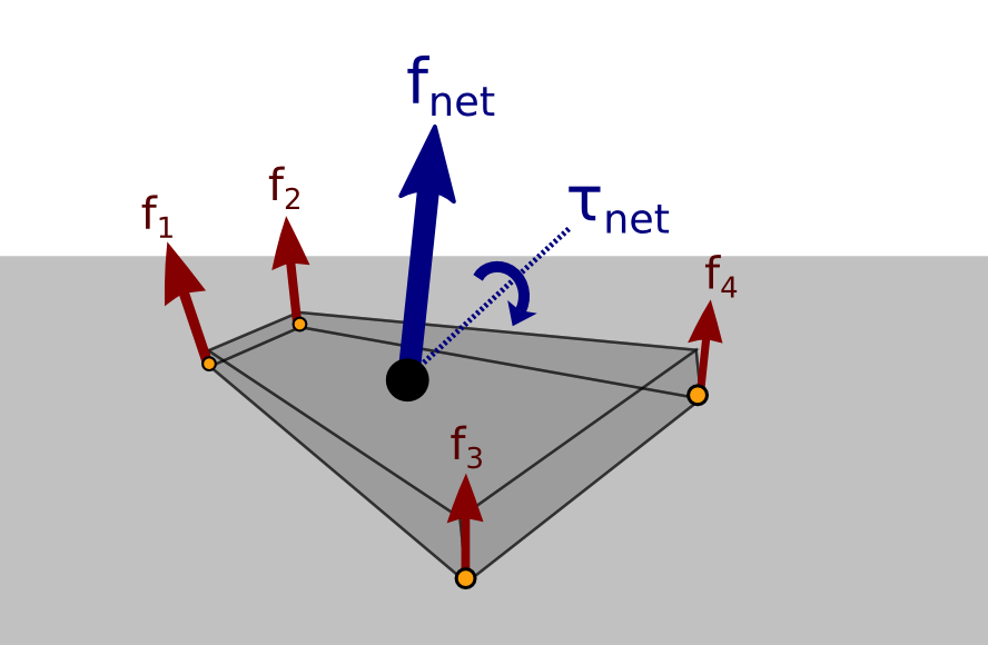
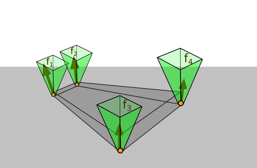
The contact force $f_{i}$ at the contact $(C_{i}, n_{i})$ has two components:

Pressure (normal): $p_{i} = (f_{i} \cdot n_{i})$
Friction (tangential): $f_{i}^{t} = f_{i} - p_{i} n_{i}$

Coulomb friction

Each surface-to-surface contact $(C_{i}, n_{i})$ yields friction, represented by a friction coefficient $μ_{i}$ and its corresponding friction cone.

Contact stability

Contact forces $f_{i}$ should lie inside their friction cones to avoid transitions towards other contact modes (e.g. sliding).

Friction and contact points

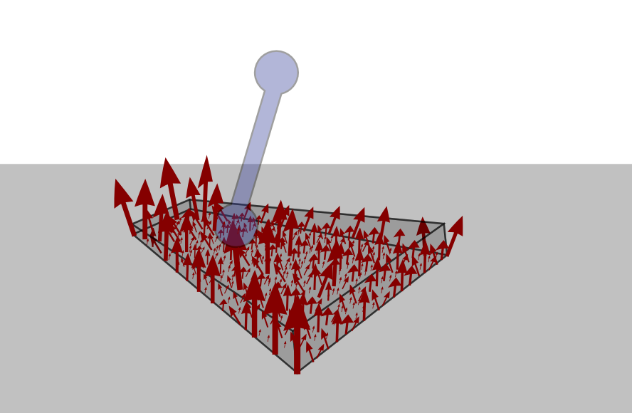
The reality of contact is a continuous distribution of infinitesimal forces.	Forces at the boundary of the contact area generate the same wrench on the rigid body.
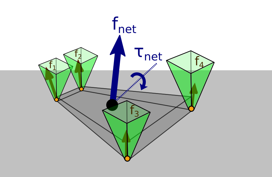
Infinitesimal Coulomb friction constraints aggregate as boundary frictions cones, usually linearized into pyramids.	How do these friction cones constraint the contact wrench? Is there a “wrench friction cone”?

Contact Wrench Cone ^{(ICRA 2015)}

Friction can be equivalently expressed by a Contact Wrench Cone (CWC):

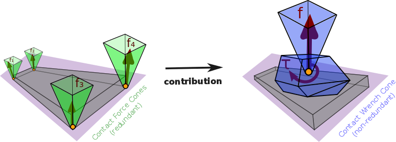
We derived the analytical formula of the CWC for rectangular contact surfaces (foot shape of current humanoids). There is therefore no additional cost in using this minimal, non-redundant representation.

Structure of the CWC

Friction Cone (4 inequalities)

The resultant force $f$ lies in a friction cone: $| f_{x} |, | f_{y} | \leq μ f_{z} \land f_{z} > 0$ .

Center of pressure (4 inequalities)

Keeps the COP in the contact polygon: $| τ_{x} | \leq Y f_{z} \land | τ_{y} | \leq X f_{z}$ .

Yaw constraints (8 inequalities)

An original discovery of our study:

\begin{matrix} τ_{z} & \in & [τ_{min}, τ_{max}] τ_{min} & := & - μ (X + Y) f_{z} + | Y f_{x} - μ τ_{x} | + | X f_{y} - μ τ_{y} |, τ_{max} & := & + μ (X + Y) f_{z} - | Y f_{x} + μ τ_{x} | - | X f_{y} + μ τ_{y} | . \end{matrix}

Corroborates works ^{(Cisneros et al., 2014)} on foot yaw regulation for humanoids.

Application to a one-foot motion

The CWC enables the use of TOPP. Below are two retimings of the same input:

CWC enforced

CWC not enforced

Multi-contact Whole-body Motions

Dynamic equilibrium

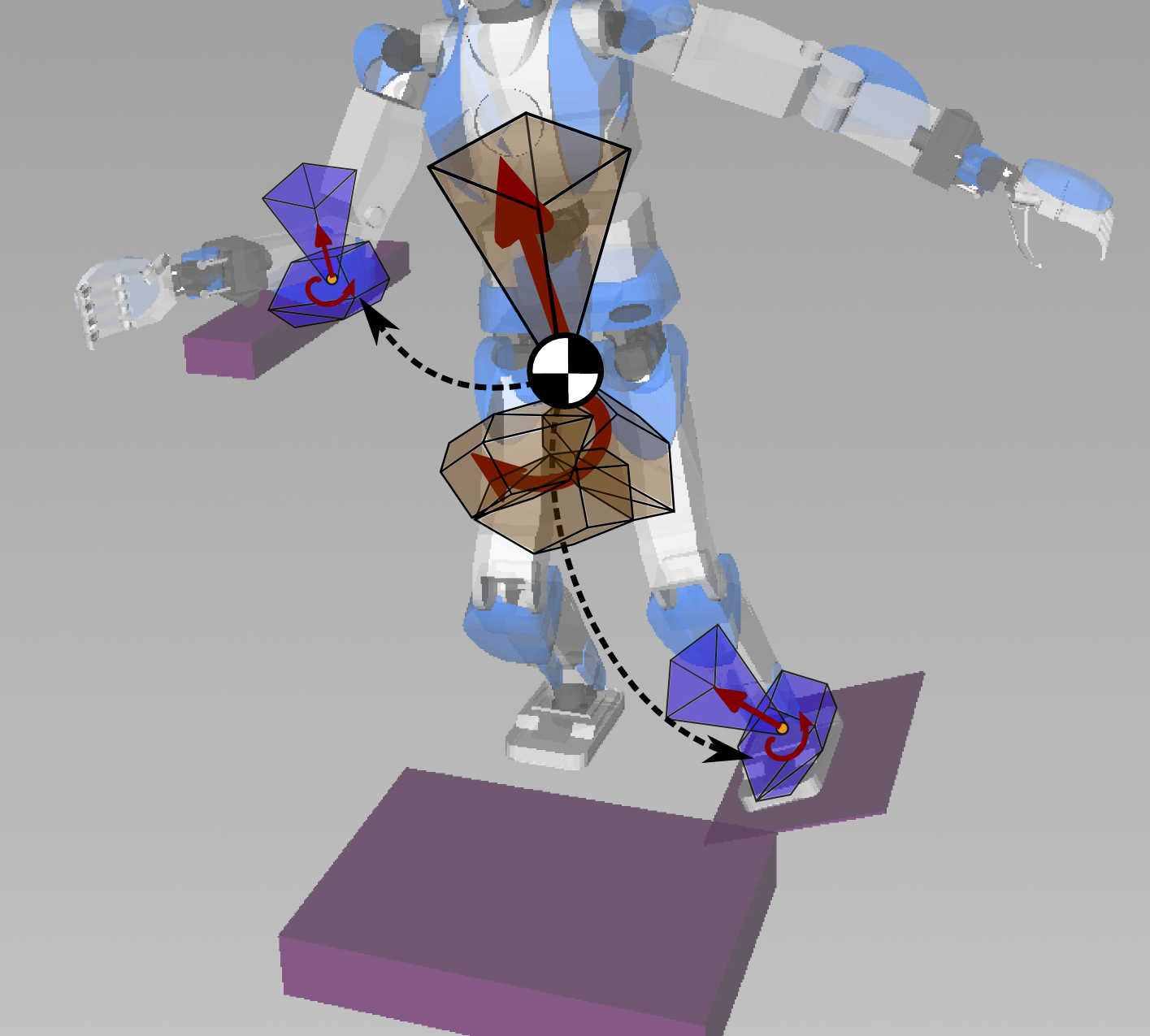
Contact forces and the centroidal momentumof the system are bound by the relation:

[\begin{matrix} m {¨ x}_{G} {˙ L}_{G} \end{matrix}] = [\begin{matrix} m g 0 \end{matrix}] + \sum c o n t a c t i [\begin{matrix} f_{i} {- - \to G C}_{i} \times f_{i} \end{matrix}]

$m$ and $g$ : total mass and gravity vector
${¨ x}_{G}$ : acceleration of the center of mass (COM)
${˙ L}_{G}$ : rate of change of the angular momentum
$f_{i}$ : contact force at $(C_{i}, n_{i})$

See e.g. (Wieber, 2008) for a proof of this result.
It derives from the assumption that internal forces are conservative (d'Alembert's principle).

Gravito-inertial wrench

The previous equation of motion rewrites to

[\begin{matrix} f^{g i} τ_{O}^{g i} \end{matrix}] := - \sum c o n t a c t i [\begin{matrix} f_{i} {- - \to G C}_{i} \times f_{i} \end{matrix}]

That is to say, $w_{O}^{g i} = A_{O}^{g i} f$ , where $w^{g i}$ is the gravito-inertial wrench. Meanwhile, four-sided linearized friction cones can be written:

⎡ ⎢ ⎢ ⎢ ⎢ ⎢ ⎣ \begin{matrix} + \sqrt{2} & 0 & - μ - \sqrt{2} & 0 & - μ 0 & + \sqrt{2} & - μ 0 & - \sqrt{2} & - μ \end{matrix} ⎤ ⎥ ⎥ ⎥ ⎥ ⎥ ⎦ R_{i}^{⊤} f_{i} \leq 0

Question: what is the image of inequalities $B f \leq 0$ by the linear mapping $w = A f$ ?

Bits of Convex Polyhedra Theory

Definitions

Minkowski sum of two sets: $P + Q = {p + q : p \in P and q \in Q}$ .
Convex hull: $c o n v (v_{1}, \dots, v_{n}) = \sum_{i} α_{i} v_{i}$ where $\forall i, α_{i} > 0$ and $\sum_{i} α_{i} = 1$ .
Positive span: $n o n n e g (r_{1}, \dots, r_{s}) = \sum_{i} λ_{i} r_{i}$ where $\forall i, λ_{i} > 0$ .

Theorem (Minkowski-Weyl)

For a subset $P$ of $R^{d}$ , the following statements are equivalent:

$P$ is a polyhedron: $P = {x : A x \leq b}$ for $A \in R^{m \times d}$ and $b \in R^{m}$
There are finite real vectors $v_{1}, v_{2}, \dots, v_{n}$ and $r_{1}, r_{2}, \dots, r_{s}$ in $R^{d}$ such that $P = c o n v (v_{1}, v_{2}, \dots, v_{n}) + n o n n e g (r_{1}, r_{2}, \dots, r_{s})$ .

Thus, every polyhedron has two representations of type (1) and (2), known as (halfspace) H-representation and (vertex) V-representation, respectively.

Adapted from the Polyhedral Computation FAQ.

Friction Cone Duality

Double-description method (Fukuda, 1996)

Libraries such as cdd (C++) and pycddlib (Python) allow for efficient conversion between H- and V-representations. In particular, for cones:

$B^{S}$ : span matrix of the cone: $B x \leq 0 \Leftrightarrow x = B^{S} λ, λ > 0$
$A^{F}$ : face matrix of the cone: $x = A λ, λ > 0 \Leftrightarrow A^{F} x \leq 0$

Derivation of the Gravito-inertial Wrench Cone (GIWC) (Qiu et al., 2011)

Dynamic equilibrium $w_{O}^{g i} = A_{O}^{g i} f$ and frictional constraints $B f \leq 0$
Conversion to span form: $f = B^{S} λ, λ > 0$
V-representation of the GIWC: $w_{O}^{g i} = A_{O}^{g i} B^{S} λ, λ > 0$
Finally, H-representation of the GIWC: $(A_{O}^{g i} B^{S})^{F} w_{O}^{g i} \leq 0$

App. to Statics and Dynamics ^{(RSS 2015)}

On top of this derivation, we applied the GIWC to two problems:

Statics: robust equilibrium

Statically stable postures that can resist bounded disturbance forces.

Dynamics: trajectory retiming

Combine the GIW with Time-Optimal Path Parameterization (TOPP library) to generate dynamic motions.

Application to Box Climbing

GIWC enforced

GIWC not enforced

Off-ground ZMP support areas
for locomotion on uneven terrains

Zero-tilting Moment Point

“Zero” Moment Point (ZMP)

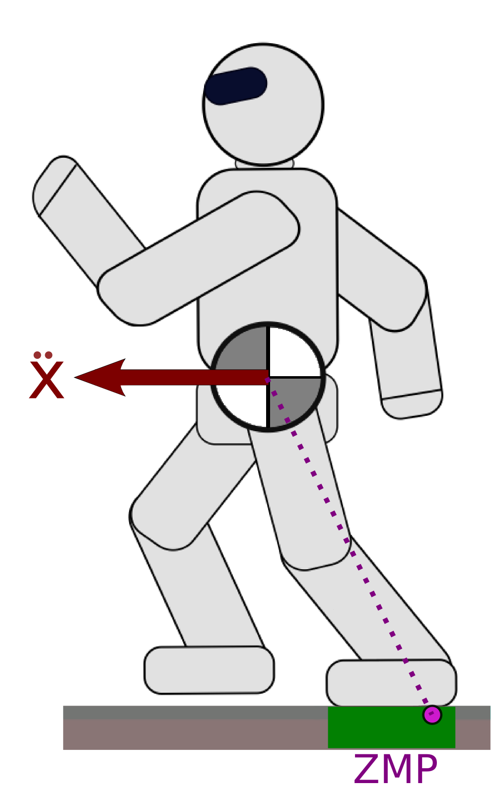
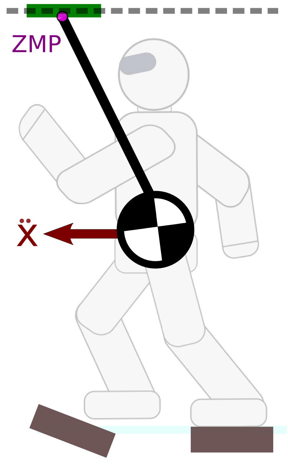
Previous definition: the point on the floor where the moment of the gravito-inertial wrench is vertical. ^{(Sardain & Bessonnet, 2004)}

Stability criterion (Vukobratovic & Stepanenko, 1972)

If the motion is dynamically balanced by valid contact forces, the ZMP lies in the convex hull of ground contact points.

Nota Bene

The resultant moment is not zero at the ZMP (it is aligned with the ground normal).

Pendular locomotion

A pendular model is (a particular mode) embedded in the equations of motion.^{(Kajita et al., 2001)} Indeed, the dynamic equilibrium equation implies that:

{¨ x}_{G} = \frac{g + {¨ z}_{G}}{z_{G} - z_{Z}} (x_{G} - x_{Z}) - \frac{{˙ L}_{G y}}{m (z_{G} - z_{Z})}

and similarly for

{¨ y}_{G}

Linear Inverted Pendulum (LIP)

Regulating ${˙ L}_{G} = 0$ , ${¨ x}_{G} = ω^{2} (x_{Z} - x_{G}),$ where $ω := \sqrt{\frac{g + {¨ z}_{G}}{z_{G} - z_{Z}}} .$

ZMP of a Wrench

Limitations

The ground ZMP can only be used for locomotion on horizontal floors
It accounts for pressure $(p_{i} > 0)$ but not for friction limits $(∥ f_{i}^{t} ∥ \leq μ_{i} p_{i})$

ZMP of a wrench (existing definition)

The ZMP is actually defined ^{(Sardain & Bessonnet, 2004)} for any wrench $w = (f, τ)$ in any virtual plane $Π (O, n)$ . The ZMP $Z \in Π (O, n)$ is the point such that $n \times τ_{Z} = 0$ :

x_{Z} = \frac{n \times τ_{O}}{n \cdot f} + x_{O} .

Full support area (new definition)

The full support area $S$ of the ZMP in the plane $Π (O, n)$ is the image of the complementary wrench cone by the equation above.

Vertices of the Full Support Area

Previous intuitions

Previous works ^{(Sugihara et al., 2002)

(Popovic et al., 2005)

(Harada et al., 2006)} tried to extend the definition as convex hull of contact point, thus looking for convex polyhedra.

Our approach

Vertices are located at the intersection of the plane with friction cones (= contact points on horizontal floor, but not in general).

x_{Z_{i}} := \frac{n \times τ_{O, i}}{n \cdot f_{i}} + x_{O} = \frac{n \times (- - \to O C_{i} \times f_{i})}{n \cdot f_{i}} + x_{O},

We will sort these vertices into two polygons:

positive (virtual) pressure $P^{+} = {x_{Z_{i}} | (n \cdot f_{i}) > 0}$ , and
negative (virtual) pressure $P^{-} = {x_{Z_{i}} | (n \cdot f_{i}) < 0}$ .

Geometric Construction

Case 1: polygon

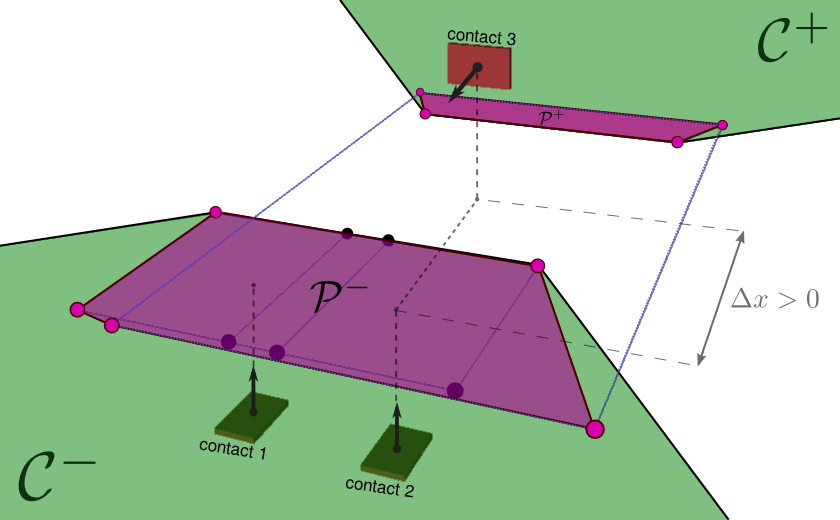
If one of the two polygons $P^{+}$ or $P^{-}$ is empty, $S$ is equal to the other.

Case 2: complementary cones

Let $D := P^{+} - P^{-} = c o n v ({r_{1}, \dots, r_{k}})$ denote the vertices of the Minkowski difference. The support area $S$ is the reunion of two polygonal cones: $C^{+} = P^{+} + \sum_{i} R^{+} r_{i}$ and $C^{-} = P^{-} + \sum_{i} R^{+} (- r_{i})$ . In particular, when $P^{+} \cap P^{-}$ has non-empty interior, $S$ covers the whole plane $Π (O, n)$ .

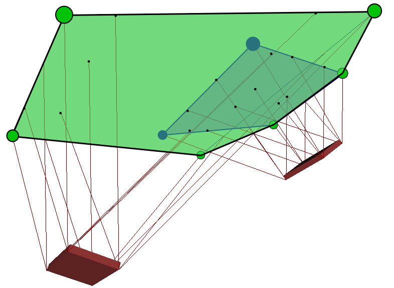
Multi-contact pendular locomotion

Now, we know how to compute the ZMP support area in any virtual plane, including those above the robot. With the latter, we get a:

Linear (non-inverted) Pendulum (LP)

The control law equation becomes ${¨ x}_{G} = ω^{2} (x_{G} - x_{Z}),$ where this time $ω := \sqrt{\frac{g + {¨ z}_{G}}{z_{G} - z_{Z}}} .$

Stability discussion

LIP: the ZMP is a repellor of the COM
LP: the ZMP is a marginal attractor of the COM

Pendular means smaller support

Even on a horizontal floor, the support area is smaller than the convex hull of ground contact points.

Angular momentum

The linear pendulum (LP or LIP) model assumes that $˙ L = 0,$ i.e., the angular momentum is regulated to a constant value.

Distance from plane

Previous works also assume ${¨ z}_{G} = 0$ , i.e., the COM is regulated to lie in a plane.

Unexpected consequence

Although it was previously unnoticed, these regulations constraint the GIWC, and therefore shrink the ZMP support area.

Pendular support area

Contribution

A novel algorithm based on the double-description method to compute the pendular support area (after shrinking due to $˙ L = 0$ and ${¨ z}_{G} = 0$ ).

Implementation

Integration within a COM-ZMP trajectory generator and validation in simulations.

Outcome

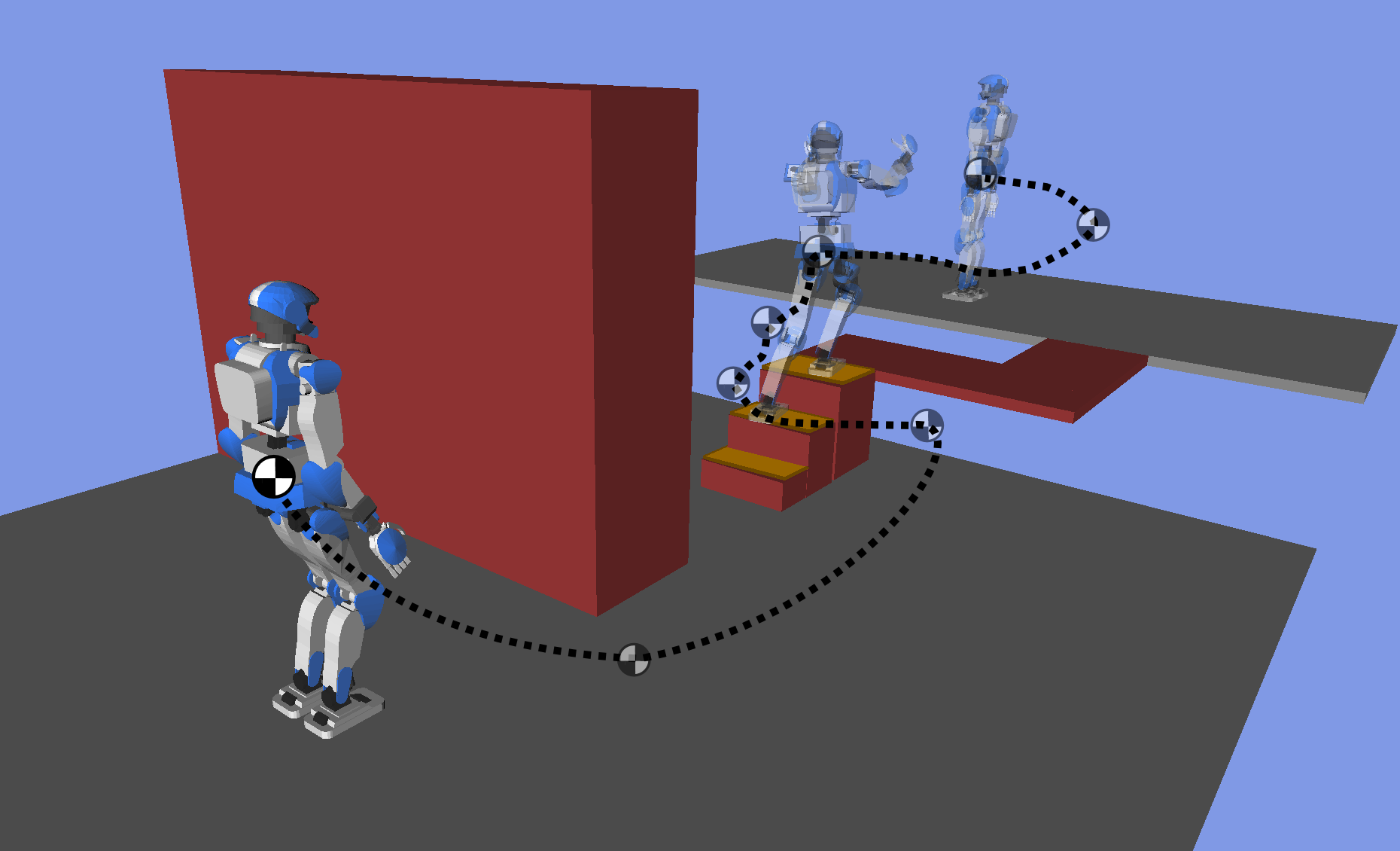
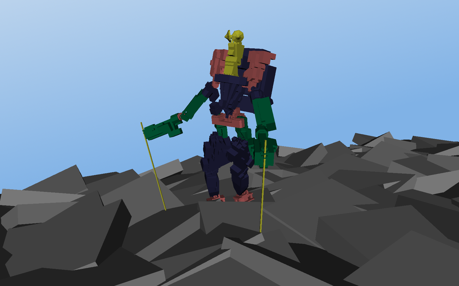
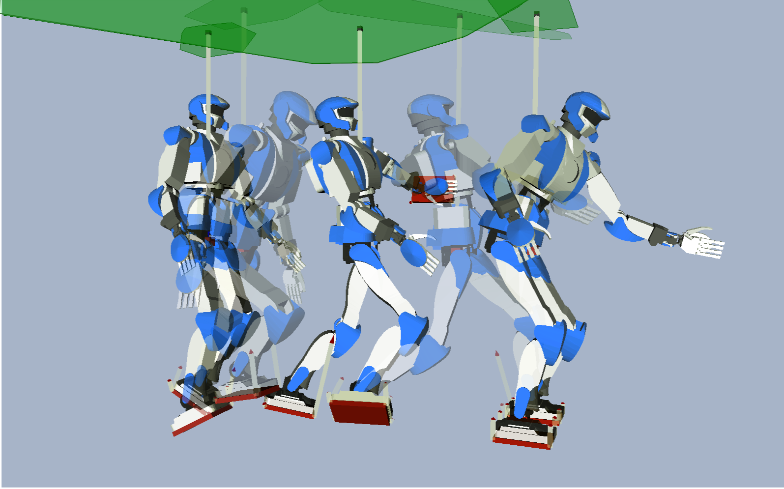
Contact-feasible whole-body multi-contact locomotion across uneven terrain.

Journey

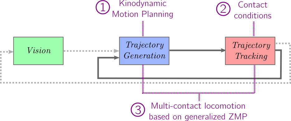
The steering idea of putting motion planning into the fast feedback loop took us in a journey through:

Overall system

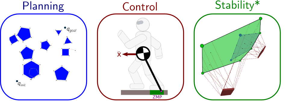
The components we described integrate with each other as follows:

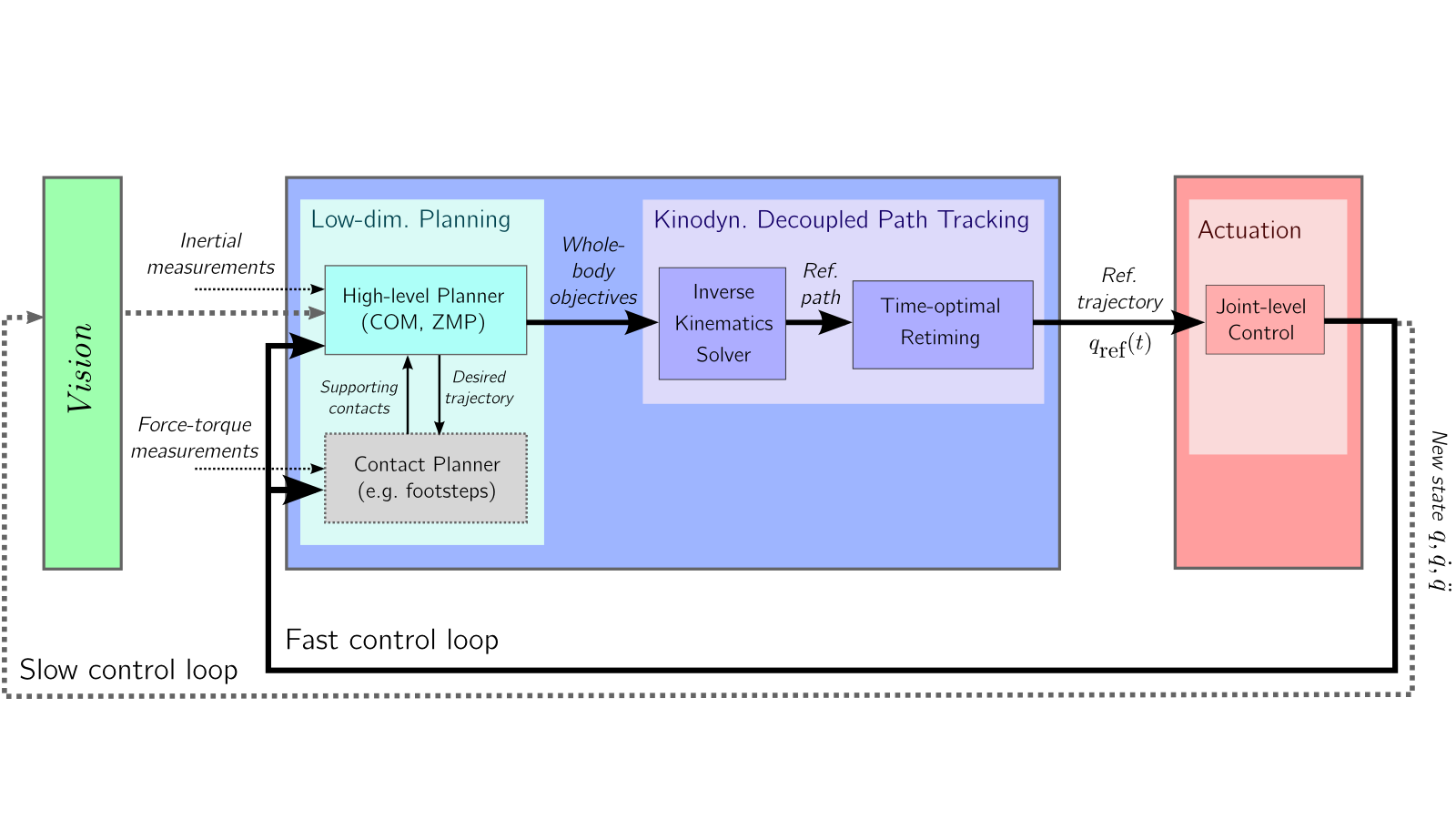
Always a great deal of open questions. For instance, what about contact planning?
The road ahead opens to many more journeys!

御清聴有り難う御座います。

Stéphane Caron – March 7^th, 2016

Perspectives on Motion Planning and Control for Humanoid Robots in Multi-contact Scenarios

Motivation

Scope

Challenges

The Feedback loop

Ideal model

State of the art

The Feedback loop (cont'd)

Enters non-holonomy

How to attack the problem

Kinodynamic Motion Planning

Motion Planning

Terminology

Property

Kinematic Motion Planning

Roadmap Planners

Idea

Approach

Stochastic Roadmap Planners

Probabilistic Roadmaps (PRM)

Rapidly-exploring Random Trees (RRT)

Completeness

Completeness

Probabilistic completeness

A correctness guarantee

Completeness of Kinematic Planners

Theorem (Kavraki et al., 1998)

Theorem (LaValle and Kuffner, 2000)

Kinodynamic Planning

Completeness of Kinodyn. Planners

Steering functions

Analytical steering

Control-based steering

State-based steering

Completeness guarantee (ICRA 2014)

Theorem

Acceleration compliance

Comparison in simulations

System

Results

Planning in space and time

State Space

Definition

Structure

Interpolation

Decoupling of the state space

Ideally

Time-Optimal Path Parameterization (TOPP)

Initial limits of TOPP

Switching contact dynamics

Integration with motion planning

Velocity Propagation (RSS 2013)

Admissible Velocity Propagation

AVP-RRT planner

Completeness guarantee

Experiments

System

Comparison to state-space planners

Friction and contact constraints

Friction

Coulomb friction

Contact stability

Friction and contact points

Contact Wrench Cone (ICRA 2015)

Structure of the CWC

Friction Cone (4 inequalities)

Center of pressure (4 inequalities)

Yaw constraints (8 inequalities)

Application to a one-foot motion

CWC enforced

CWC not enforced

Multi-contact Whole-body Motions

Dynamic equilibrium

Gravito-inertial wrench

Bits of Convex Polyhedra Theory

Definitions

Theorem (Minkowski-Weyl)

Friction Cone Duality

Double-description method (Fukuda, 1996)

Derivation of the Gravito-inertial Wrench Cone (GIWC) (Qiu et al., 2011)

Completeness guarantee ^{(ICRA 2014)}

Velocity Propagation ^{(RSS 2013)}

Contact Wrench Cone ^{(ICRA 2015)}

App. to Statics and Dynamics ^{(RSS 2015)}

Off-ground ZMP support areas
for locomotion on uneven terrains