Time-Optimal Path Param.: a tool for Humanoid Motion Planning and Predictive Control

Stéphane Caron
LIRMM, CNRS-UM2
Talk at Humanoids 2016, W3
November 15, 2016
https://scaron.info/slides/humanoids-2016/

In this talk...

Time-Optimal Retiming

Kino-dynamic process

1. Interpolate a path $s\mapsto q\left(s\right)$
2. Find a path retiming $t\mapsto s\left(t\right)$

Disclaimer

It is not for time optimality that we use time-optimal retiming.

Manipulator

(for starters)

Full dynamics

Equations of motion for a fixed-base manipulator:

subject to torque constraints $|\tau |\le {\tau }_{max}$.

Path-tracking dynamics

The robot tracks the path $s\mapsto q\left(s\right)$ retimed as $s\left(t\right)$:

Torque constraints can then be written as  $a\left(s\right)\ddot{s}+b\left(s\right){\dot{s}}^2+c\left(s\right)\le 0$.

Time-optimal solutions

TOPP applies to all systems for which path-tracking constraints can be written:

Pontryagin's maximum principle

At each $s\left(t\right)$ of the retimed trajectory:

• either $\ddot{s}$ is maximal: $\ddot{s}=\beta (s,\dot{s})$
• or $\ddot{s}$ is minimal: $\ddot{s}=\alpha (s,\dot{s})$

We know how to enumerate switch points where the optimal solution alternates between $\alpha$ and $\beta$ [Pham, TRO 2014].

Phase Space

Waiter motion

Source: CRI group @ NTU.

Whole-body Optimization

Whole-body dynamics

The equations of motion for a humanoid are:

with separate constraints:

• torque limits:  $|\tau |\le {\tau }_{max}$
• linearized friction cones:  $A_i{f}_i\le 0$

Question

How to write them as $a\left(s\right)\ddot{s}+b\left(s\right){\dot{s}}^2+c\left(s\right)\le 0$?

Tour de force

Solution found by [Hauser, IJRR 2014]:

• Eliminate torque variables:
$$\tau (s,\dot{s},\ddot{s})=m\left(s\right)\ddot{s}+c\left(s\right){\dot{s}}^2+g\left(s\right)-\sum J_i^{\top }\left(s\right)f_i$$
• Constraints are now a polytope  $B[\ddot{s}{\dot{s}}^{2}F{]}^{\top }\le d$, where $F$ stacks contact forces.
• Project all force variables [Bretl and Lall, TRO 2008] to get a polygon: $$a\ddot{s}+b{\dot{s}}^2+c\le 0$$

Figure adapted from [Hauser, IJRR 2014].

Certificate of feasibility

Forces are not explicitely computed by the optimizer.

Yet, we have the guarantee that the controller can find feasible forces at run time.

Experiments

[Pham & Stasse, TMECH 2015] improved the algorithm for numerical TOPP.

Source: CRI group @ NTU.

Time to run TOPP on $N=100$ discretization steps: $5ms$
versus $2.5s$ with non-linear optimization (SLP).

How can a “time optimal” motion
be so slow?

Answer: Robustness

All dynamic constraints are scaled:

• Torques: $|\tau |\le {\gamma }_{\tau }{\tau }_{max}$
• Friction: $|f_i^t|\le {\gamma }_f\mu f_i^z$
• Area of surface contacts scaled by ${\gamma }_s$

where ${\gamma }_{\tau },{\gamma }_f,{\gamma }_s\in (0,1)$, typically 50%.

Bottlenecks

Question 1

Most computation time ($\sim 1s$) is now spent computing $a\left(s\right),b\left(s\right),c\left(s\right)$.

Question 2

What to update in a joint-angle path $q\left(s\right)$ when there is no solution?

Reduced-model Optim.

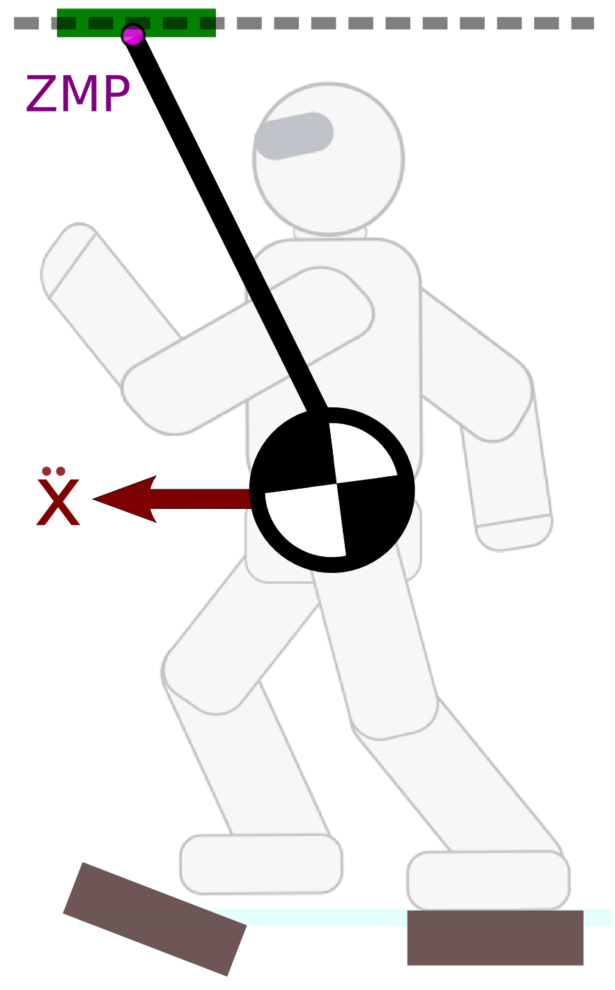
Contact Wrench Cone

Rationale

In multi-contact, frictional constraints are way more critical than torque limits.

Definition

Friction cone of resultant contact wrench.

Reduced model

Center of mass + Angular momentum.

Pipeline

We don't know how to interpolate the angular momentum, therefore:

Discussion

• Whent it fails: update the COM path.
• Can we avoid the IK step for the angular momentum?
  (e.g. using the Linear Pendulum Mode where ${\dot{L}}_G=0$)

Reduced-model Support Polytopes

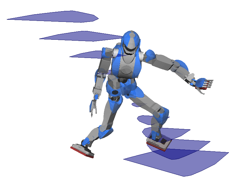
Multi-contact ZMP support areas
[Caron et al., TRO 2016]

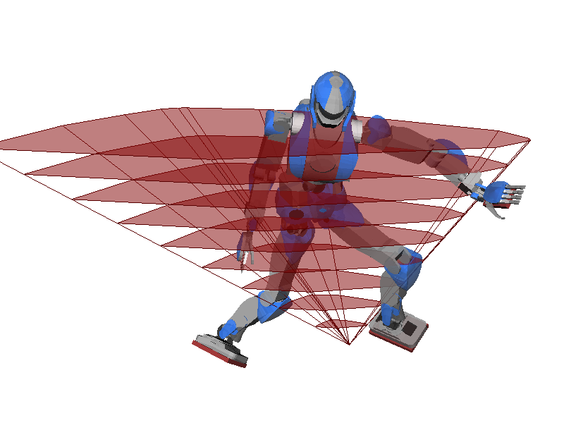
COM acceleration support volume
[Caron et al., Humanoids 2016]

Predictive Control

Step timings

Fixed step timings do not work any more in multi-contact, where proper timings depend on terrain topology.

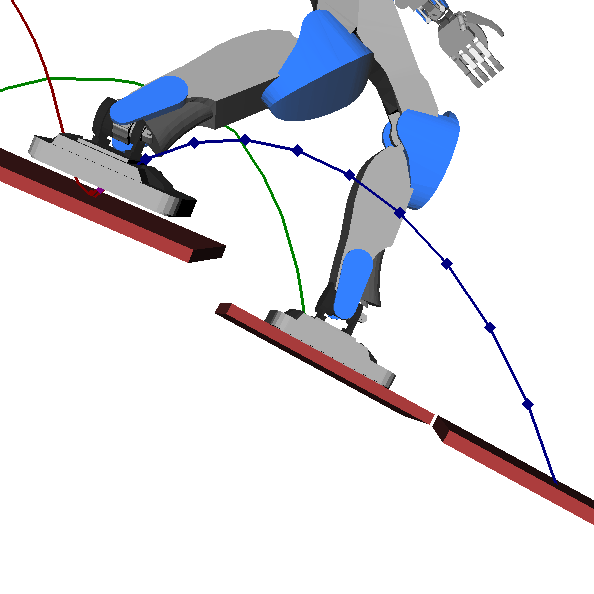
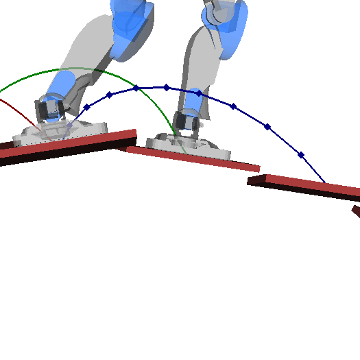
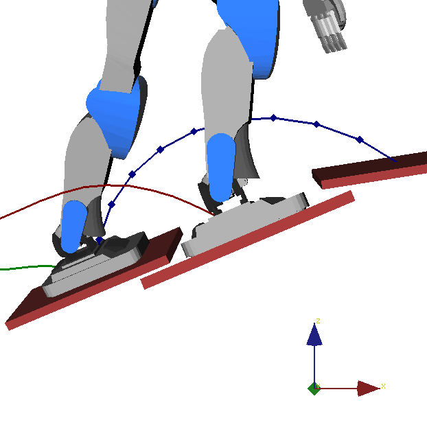
Multi-contact MPC on 3D COM

TOPP-MPC

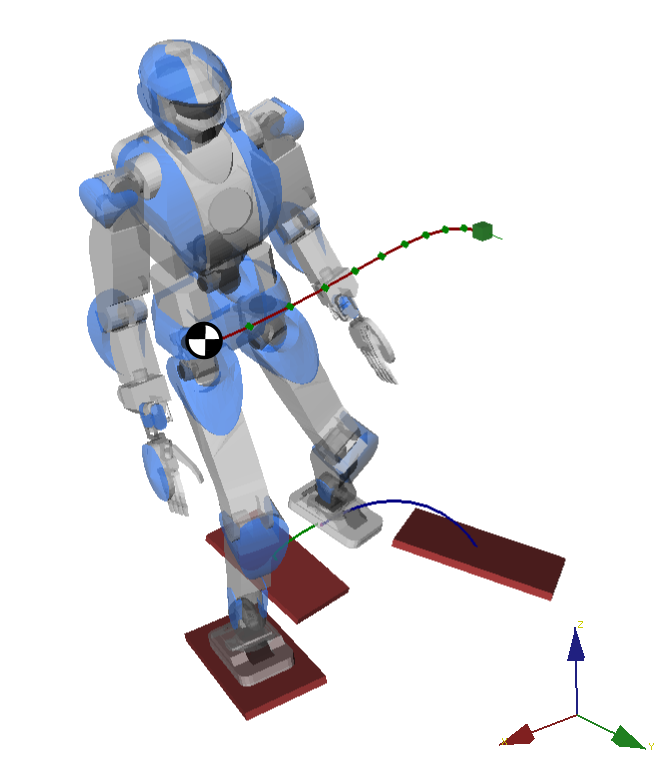
Ongoing work with Quang-Cuong Pham.

Idea

Use TOPP as dynamics filter in a predictive controller.

Main benefit

Step timings are computed automatically.

Contact switch in preview window

Parameterize foot trajectory, feed back step timing to COM optimization.

Pipeline

Continuous interpolation/retiming loop running at 20-30 Hz.

https://github.com/stephane-caron/topp-mpc

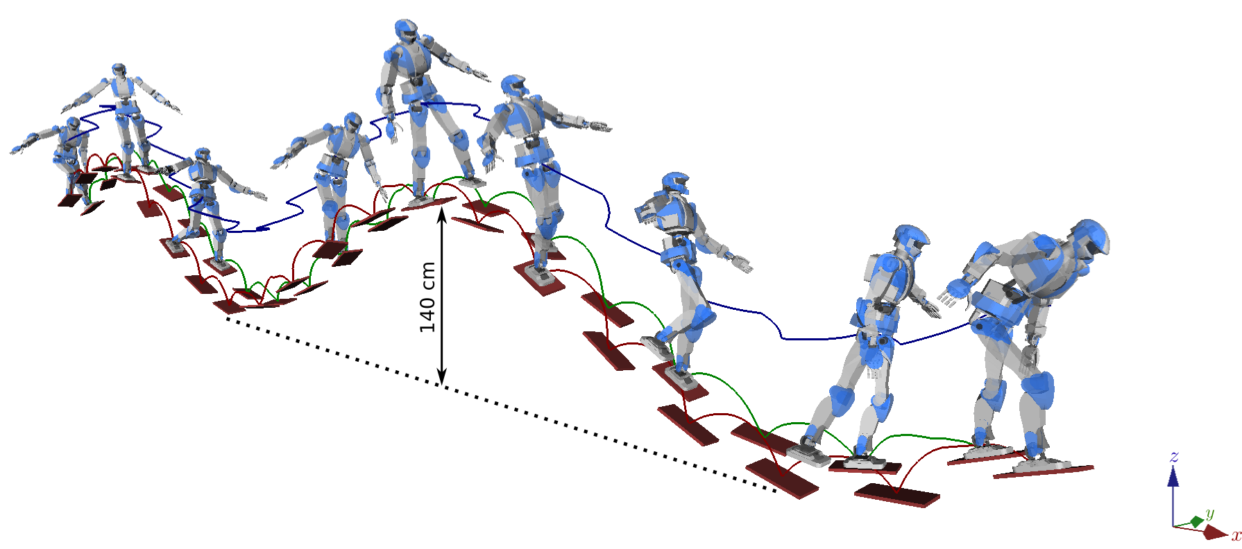
Concluding remarks

Time-optimal retiming

A fast dynamics filter.

Whole-body TOPP

Core idea of polytope projection: force/torques are not explicitly computed.

Reduced-model TOPP

Low-dimensional model for replanning and faster computations.

Predictive control

Nonlinear optimization running at 20-30 Hz in the control loop.