Examples

Triple integrator

Let us define a triple integrator:

import numpy as np

horizon_duration = 1.0
nb_timesteps = 16
T = horizon_duration / nb_timesteps
A = np.array([[1.0, T, T ** 2 / 2.0], [0.0, 1.0, T], [0.0, 0.0, 1.0]])
B = np.array([T ** 3 / 6.0, T ** 2 / 2.0, T]).reshape((3, 1))

Suppose for the sake of example that acceleration is the main constraint acting on our system. We thus define an acceleration constraint |acceleration| <= max_accel:

max_accel = 3.0  # [m] / [s] / [s]
accel_from_state = np.array([0.0, 0.0, 1.0])
ineq_matrix = np.vstack([+accel_from_state, -accel_from_state])
ineq_vector = np.array([+max_accel, +max_accel])

This leads us to the following linear MPC problem:

from qpmpc import MPCProblem

initial_pos = 0.0
goal_pos = 1.0
problem = qpmpc.MPCProblem(
    transition_state_matrix=A,
    transition_input_matrix=B,
    ineq_state_matrix=ineq_matrix,
    ineq_input_matrix=None,
    ineq_vector=ineq_vector,
    initial_state=np.array([initial_pos, 0.0, 0.0]),
    goal_state=np.array([goal_pos, 0.0, 0.0]),
    nb_timesteps=nb_timesteps,
    terminal_cost_weight=1.0,
    stage_state_cost_weight=None,
    stage_input_cost_weight=1e-6,
)

We can solve it with:

from qpmpc import solve_mpc

plan = solve_mpc(problem, mpc)

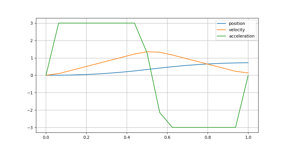
The resulting plan holds complete state and input trajectories as stacked vectors. For instance, we can plot positions, velocities and accelerations as follows:

import pylab

t = np.linspace(0.0, horizon_duration, nb_timesteps + 1)
X = plan.states
positions, velocities, accelerations = X[:, 0], X[:, 1], X[:, 2]
pylab.ion()
pylab.plot(t, positions)
pylab.plot(t, velocities)
pylab.plot(t, accelerations)
pylab.grid(True)
pylab.legend(("position", "velocity", "acceleration"))

This example produces the following trajectory:

The behavior is a weighted compromis between reaching the goal state (weight 1.0) and keeping reasonable finite jerk inputs (weight 1e-6), which prevents bang-bang accelerations.